
Long Short-Term Memory Recurrent Neural Network-Based Acoustic Model Using Connectionist Temporal Classification on a Large-Scale Training Corpus
2017-04-09 05:52DonghyunLeeMinkyuLimHosungParkYosebKangJeongSikParkGilJinJangJiHwanKim
China Communications 2017年9期
Donghyun Lee, Minkyu Lim, Hosung Park, Yoseb Kang, Jeong-Sik Park, Gil-Jin Jang, Ji-Hwan Kim,*
1 Department of Computer Science and Engineering, Sogang University 35 Baekbeom-ro, Mapo-gu,Seoul, 04107, Republic of Korea
2 Department of Information and Communication Engineering, Yeungnam University 280 Daehak-Ro,Gyeongsan, Gyeongbuk, 38541, Republic of Korea
3 School of Electronics Engineering, Kyungpook National University 80 Daehakro, Bukgu, Daegu, 41566,Republic of Korea
* The corresponding author, email:kimjihwan@sogang.ac.kr
I. INTRODUCTION
Speech recognition is a human-computer interaction technology that can control various devices and services such as smartphones by using a human speech without a keyboard or a mouse [1]. A representative application of speech recognition is an intelligent personal assistant (IPA) such as Apple’s Siri. In addition, Baidu and Google provide search engines using speech recognition [2][3].
The goal of speech recognition technologies is to estimate word sequences from the human speech by using an Acoustic Model (AM) and a Language Model (LM), which are statistical models [4].

Equation (1) applies the Bayesian theory to calculate the word sequence W (which is the most similar to a given word sequence spokenby a person) from an acoustic vector O for. P(O) is a probability for the acoustic vector and it was removed in (1) because it is independent to W. Thus, the product of P(W) and P(O|W) is calculated for all possible cases. W is returned as the result of speech recognition.P(W) and P(O|W) are estimated from the LM and the AM, respectively.
The LM provides information about the syntax between words in the word sequence W. An N-gram is a training method for generating LM. It models the relationships between words using word frequencies from a text corpus. The AM is to model speech units using acoustic vectors extracted from given speech signals. The acoustic model based on Gaussian Mixture Model (GMM)-Hidden Markov Model (HMM) expresses the observation probability from each state of the HMM in the training corpus [5][6].
Recently, methods using deep learning for generating LMs and AMs show a higher performance than previous methods. A LM based on Recurrent Neural Network (RNN) using word vectors that express words as vectors is applied to N-gram rescoring and shows a higher performance than the N-gram language model [7][8][9]. An AM based on Deep Neural Network (DNN) shows a higher performance than the GMM-HMM-based AM. Furthermore, an AM based on Long Short-Term Memory (LSTM) RNN has proposed and improved on the performance of the DNNHMM-based AM [10][11][12].
However, a hybrid method that models the observation probability of HMM using DNN or LSTM RNN uses supervised learning, and thus requires a forced-aligned HMM state sequence for each acoustic vector from the GMM-HMM-based AM. This method has problems as follows: 1) The GMM-HMM-based acoustic model have to be trained before training the DNN-HMM-based AM because the most of the AM training corpus only provides speech data and word-unit scripts, 2)the hybrid method is time-consuming because both the GMM-HMM-based AM and the DNN-HMM-based AM have to be trained, 3)incorrect alignment data is provided because the forced-aligned HMM state sequence is obtained from the GMM-HMM-based AM statistically rather than from a person.
To solve these problems, an AM using Connectionist Temporal Classification (CTC),which is an end-to-end (or sequence-to-sequence) method, is proposed [13][14][15].CTC is an objective function of output nodes in an output layer of a given deep learning model. In CTC algorithm, output nodes are mapped to a phoneme or a character used in target language, and a phoneme sequence or a character sequence is estimated by using a forward-backward algorithm.
However, previous research for AMs using CTC has used only the small-scale corpus, and the performance of AMs using CTC has not evaluated for the large-scale corpus. In this paper, the LSTM and CTC algorithms are analyzed, and an LSTM RNN-based AM using CTC is trained with the large-scale training corpus. Then, a performance of the proposed AM is compared with DNN-HMM-based AM trained by the hybrid method.
The composition of this paper is organized as follows. In Section II, the LSTM architecture and CTC algorithm are analyzed through previous works. In Section III, the LSTM RNN-based AM using CTC is trained with the large-scale English training corpus, and its performance is compared with that of the DNN-HMM-based AM. In Section IV, the conclusion is presented.
II. RELATED WORKS
2.1 LSTM Architecture
In DNN models, vanishing gradient problem is occurred. It is the problem that the error rate converges to zero when error back-propagation is performed. Furthermore, when error back-propagation is performed in RNNs, the error rate of the hidden layer at time (t-1) is reflected in the error rate of the hidden layer at time t, and the error rate converges to zero continuously as time t increases for input data with a long context.
In order to solve vanishing gradient problem, the LSTM architecture was applied to the hidden node. LSTM is a hidden node structure, as shown in figure 1. It consists of one or more memory cells, an input gate, an output gate, and a forget gate [16][17][18]. As a result, the error rate did not converge to zero by the memory cell of LSTM even in a long context.


Fig. 1 Architecture of LSTM-based hidden node
Equation (2) is an equation for the input gate igtin figure 1. Wx,igis a weight matrix between a input vector xtand the input gate,Who,igis a weight matrix between the hidden node and the input gate at time (t-1), Wmc,igis a weight matrix between the memory cell and the input gate at time (t-1), hot-1is the output value of the hidden node at time (t-1), mc(t-1)is the output value of the memory cell at time (t-1), and bigis the bias value of the input gate.
Equation (3) is an equation for the output gate ogtin figure 1. Wx,ogis a weight matrix between the input vector xtand the output gate,Who,ogis a weight matrix between the hidden node and the output gate at time (t-1), Wmc,ogis a weight matrix between the memory cell and the output gate at time (t-1), and bogis the bias value of the output gate. In the LSTM architecture, the input gate and output gate increase or decrease the error rate of the weight during the error back-propagation, thereby solving the vanishing gradient problem.
Equation (4) is an equation for the forget gate fgtin figure 1. Wx,fgis a weight matrix between the input vector xtand the forget gate,Who,fgis a weight matrix between the hidden node and the forget gate at time (t-1), Wmc,fgis a weight matrix between the memory cell and the forget gate at time (t-1), and bfgis the bias value of the forget gate. The forget gate resets the value of the memory cell to zero if the information stored in the memory cell until time(t-1) is not associated with the error signal at time t. This solves the vanishing gradient problem of RNN models.
Equation (5) is an equation for the memory cell mctin figure 1. Wx,mcis a weight matrix between the input vector xtand the memory cell,Who,mcis a weight matrix between the hidden node and the memory cell at time (t-1), and bmcis the bias value of the memory cell. The memory cell maintains the same error value regardless of time during error back-propagation for input data with a long context.
Equation (6) is an equation for the final output value of the LSTM-based hidden node at time t in figure 1. The deep learning model using this LSTM architecture requires a large amount of training corpus because LSTM-based model training has to train 3-4 times more weights than DNN-based model training. Thus, it has the problem of consuming long training time. To solve this problem, new configurations of the LSTM architecture and changes to the deep learning model architecture have been researched in recent years.
K. Cho et al. [19] proposed Gated Recurrent Unit (GRU), which simplified the LSTM architecture. GRU reduced a complexity of the LSTM architecture by decreasing three gates of the LSTM architecture to two gates,called the update gate and output gate, which perform the functions of the input and forget gates simultaneously as reset gates, respectively. Furthermore, an English-French translation based on GRU showed a higher score by 0.77 in terms of Bilingual Evaluation Understudy(BLEU) score than RNN models. BLEU score is an evaluation metric for performance of machine translation from one language to another.
K. Greff et al. [20] analyzed the LSTM architecture from various points of view with the TIMIT, IAM, and JSB Chorales corpus. In[20], the performance showed no difference in the experiment even if the input gate, output gate, or forget gate of the LSTM architecture did not exist. This is the same as the case of using the GRU in [19], which did not show performance degradation. Furthermore, the value of the learning rate was found to have a great effect on the performance of trained models when the deep learning model using LSTM was trained. However, the TIMIT,IAM, and JSB Chorales corpus are small corpora of 100 hour or less, and an analysis of the LSTM architecture with a large corpus of 1,000 hour or more was not presented.
H. Sak et al. [21] proposed a method of addition both a recurrent projection layer and a non-recurrent projection layer between the LSTM layer and the output layer. The proposed method solved the problem of high computational complexity in the recurrent hidden layer consisting of LSTM nodes. Furthermore, it showed the lowest Word Error Rate(WER) when compared with both the DNNHMM-based AM and the RNN-based AM.
2.2 CTC Algorithm
The hybrid method requires forced-aligned HMM state sequence for each acoustic feature in order to provide the correct answer because it uses supervised learning. This method has problems as follows: 1) The GMM-HMM-based AM have to be trained before training the DNN-HMM-based AM and it takes a long training time, 2) incorrect alignment data is provided because statistically forced-aligned data is obtained.
In order to solve these problems, Graves et al. [12][13][14][15] proposed an AM training method using CTC algorithm to obtain a phoneme or a character from each acoustic feature in deep learning models without training the GMM-HMM-based AM. CTC is an objective function of a output node in the output layer of given deep learning models, and each output node reflects the phoneme or character defined in the target language. When training the deep learning model using CTC, correct answer scripts are presented in word or phoneme units. Thus, the forced-aligned HMM state sequence is not required from the GMM-HMM-based AM.
For example, the number of given labels from the training corpus of target language is K. In the deep learning-based AM using CTC,the output layer is composed of (K+1) output nodes. One output node is added to reflect the empty label Ø. The empty label is used to output a meaningless label when a given acoustic feature is not associated with any of K labels.In this model architecture, CTC is trained by forming pairs of each acoustic feature and a label such as the phoneme or character automatically. In other words, as shown in (7), the CTC training procedure is progressed with a goal of finding L that is most similar to the correct answer label sequence L*from the given acoustic feature sequence X.
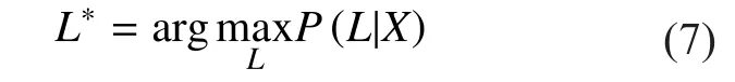
In (7), P(L|X) is identical to (8). θ is every label sequence that can be created from the set C, which has the empty label added to the set of phonemes or characters from the labels. E is a function that removes duplicate label sequences and the empty label from θ. The rule for removing duplicate labels is as follows:1) remove duplicate labels from all labels except the empty label, 2) remove the empty label. For example, when the label sequence ØaaØbaØbbØ is given as input for the function E, it is converted to E(ØaaØbaØbbØ) =abab.is the observation probability of the label corresponding to time t of θ.

For the goal of CTC, the loss function LF of the output layer at time t is applied in (9).
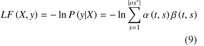
In (9), y is the sub-label sequence of L,which has taken function E for the output sequence os*, which can be generated until time t. s is the index of the output node in the output layer. α is a forward variable, which is the sum of the probabilities of all sequences for length t, which corresponds to a prefix for s/2 of L. β is the sum of the probabilities of all sequences from time (t+1) to |L| when there is a path that has determined through α. The forward-backward algorithm is used to calculate α and β. Figure 2 illustrates the forward-backward algorithm when the acoustic feature sequence X is given for length T.

Fig. 2 Forward-backward algorithm for CTC
In figure 2, white circles indicate empty labels, and black circles indicate all labels except for empty labels. Empty labels correspond to silence or short pauses at ends of the correct answer label sequence in the learning process. The label that can be selected first in the forward-backward algorithm is an empty label or one from all labels except the empty labels. Then, the label can be selected at time t (t ≥ 1) is as follows: 1) if the label selected at time (t-1) was an empty label, an empty label is selected again, or one of all labels except empty labels is selected, or 2) if the label selected at time (t-1) was one of the labels that are not empty labels, the same label is selected again, or an empty label or one of the labels except the label selected at time (t-1) and the empty labels is selected.

In [13], a bidirectional RNN-based AM using CTC was proposed. The previous RNN models were a forward RNN and could only learn the frames that appeared before the current time t at all times. It proposed a backward RNN architecture that can learn the frames that appeared after the frame at time t in advance, and also proposed an AM structure based on a deep bidirectional RNN consisted by multiple bidirectional RNN models. This AM used a tri-gram language model and showed a performance of 8.7% in terms of WER on WSJ corpus. However, the performance of the proposed model on a large-scale training corpus was not shown because the WSJ corpus is a small-scale corpus.
In [15], the performance of the LSTM RNN-based AM using CTC on the WSJ corpus showed a 0.6% error rate higher than that of the DNN-HMM-based AM in terms of WER. However, it was difficult to be shown by analyzing an accurate comparison of performance because the numbers of weight parameters of the LSTM RNN model and the DNN model were not identical. Furthermore,the performance of the LSTM RNN-based AM using CTC on a large-scale corpus was not shown because this experiment only used a small-scale corpus.
D. Amodei et al. [23] proposed a model for applying CTC to the acoustic model consisting of the Convolutional Neural Network (CNN)and the RNN using GRU with a large-scale corpus of 11,940 hour. Furthermore, it was shown that the RNN-based AM using GRU learns faster than the RNN-based AM using LSTM. In [23], the WERs were 5.33% and 13.25% for clean speech and noisy speech, respectively, which are the test set of the Libri-Speech corpus. However, the performance of this RNN model was not shown by using only RNN model because the CNN model was also used with it.
III. EXPERIMENTS AND EVALUATION
Section III describes the experiments for a performance evaluation of the LSTM RNN-based AM using CTC and the DNN-HMM-based AM on a large-scale English training corpus. Section III.A describes the experimental environment, and Section III.B describes the results of the performance evaluation.
3.1 Experimental environments
The Kaldi speech recognition toolkit was used to train AMs [24]. The Kaldi toolkit, which is based on C++, supports the various AM training methods based on deep learning, and decoding methods based on a Weighted Finite State Transducer (WFST). Furthermore, the N-gram-based LM was used for generating LMs, and the SRILM open-source toolkit was used to train LMs. The SRILM toolkit supports various training methods.
The LibriSpeech corpus was used for training AMs and LMs. This corpus is an English-read speech corpus of 1,000 hours based on audio books of LibriVox. The Kaldi supports the training method of hybrid method-based AMs using the LibriSpeech corpus.In Section III.B, the DNN-HMM-based AM is trained with the LibriSpeech corpus on Kaldi,and the performance of this model is compared with that of the LSTM RNN-based AM using CTC. In order to train the LSTM RNN-based AM using CTC, a model training code was developed by modifying source codes of LSTM RNN-based AM provided by Kaldi.
All speech corpus was recorded in 16-bit resolution at a 16kHz sampling rate and in a mono channel. Mel-Frequency Cepstral Coefficients (MFCCs) were extracted from each frame in speech corpus. The length of a frame was 25ms and the length of frame shift was 10ms. The MFCC using 40-dim features was used. It means that 40 cepstrums and 40 triangular mel-frequency bins were in the extracted MFCC.
3.2 Performance evaluation using large-scale English training corpus
The topologies of the AMs are listed in table 1. In table 1, the bidirectional RNN was used for the LSTM RNN model. Thus, it was written that a total of 10 hidden layers were used with five hidden layers each for forward RNN and backward RNN.
For the DNN-HMM model, a projection layer consisting of 500 nodes was used after a hidden layer consisting of 5,000 hidden nodes.Weights between the hidden layer and the projection layer were not updated and played the role of projecting the output value of the hidden layer. In table 1, the experiment could be performed under the assumption that a performance which is caused by the number of weights is not changed because around 12M weight parameters are used for both models.
A test set was conducted with the test corpus provided by LibriSpeech. It consists ofclean speech (6 hours) and noisy speech (6 hours). Test results are listed in table 2. When clean speech and noisy speech test data were used, a performance of the LSTM RNN-based AM using CTC was measured as 6.18% and 15.01% for clean speech and noisy speech,respectively. Even though the performance of the DNN-HMM-based AM was slightly higher in terms of WER, the performance was similar to that of the DNN-HMM-based AM when the AM was trained using only LSTM RNNs and did not used the forced-aligned data from the GMM-HMM-based AM.

Table I Topology for Acoustic Models Based on LSTM RNN and DNN-HMM

Table II WER for LSTM RNN-based Acoustic Models using CTC
IV. CONCLUSION
This paper analyzed the LSTM architecture and CTC algorithm, and the performance of the LSTM RNN-based AM using CTC was evaluated with the LibriSpeech corpus, which consists of the large-scale English training corpus. The LSTM architecture solved the vanishing gradient problem of DNNs and RNNs, but showed the problem of a long training time owing to the complexity of the structure. CTC algorithm solved these problems of the hybrid method without training the GMM-HMM-based AM. However, previous works for CTC algorithm used only the smallscale corpus such as TIMIT and WSJ corpus,and could not verify the performance of CTC algorithm with the large-scale training corpus.This paper also showed the performance of the LSTM RNN-based AM using CTC was similar to that of the DNN-HMM-based AM with large-scale training corpus as well.
ACKNOWLEDGEMENT
This material is based upon work supported by the Ministry of Trade, Industry & Energy(MOTIE, Korea) under Industrial Technology Innovation Program (No.10063424, ‘development of distant speech recognition and multi-task dialog processing technologies for in-door conversational robots’).
[1] A. Acero et al., “Live Search for Mobile: Web Services by Voice on the Cellphone,” Proc. Interspeech, pp 5256-5259, Mar., 2008.
[2] J. Jiang et al., “Automatic Online Evaluation of Intelligent Assistants,” Proc. the 24th International Conference on World Wide Web, pp 506-516, May, 2009.
[3] T. Bosse et al., “A Multi-Agent System Architecture for Personal Support during Demanding Tasks,” Proc. Interspeech, pp 1045-1048, Sep.,2010.
[4] L. Rabiner and B. Juang, “Fundamentals of Speech Recognition 1st Edition,” Prentice Hall,Apr., 1993.
[5] D. Su, X. Wu, and L. Xu, “GMM-HMM Acoustic Model Training by a Two Level Procedure with Gaussian Components Determined by Automatic Model Selection,” Proc. ICASSP, pp 4890-4893, Mar., 2010.
[6] H. Hermansky, D. Ellis, and S. Sharma, “Tandem Connectionist Feature Extraction for Conventional HMM Systems,” Proc. ICASSP, pp 1635-1638, June., 2000.
[7] T. Mikolov et al., “Recurrent Neural Network based Language Model,” Proc. Interspeech, pp 1045-1048, Sep., 2010.
[8] T. Mikolov et al., “Extensions of Recurrent Neural Network Language Model,” Proc. ICASSP, pp 5528-5531, May, 2011.
[9] T. Mikolov and G. Zweig, “Context Dependent Recurrent Neural Network Language Model,” Microsoft Research Technical Report (MSRTR-2012-92), pp 1-10, July, 2012.
[10] G. Hinton et al., “Deep Neural Networks for Acoustic Modeling in Speech Recognition,” IEEE Signal Processing Magazine, vol.29, no.6, pp 82-97, Oct., 2012.
[11] L. Deng, G. Hinton, and B. Kingsbury, “New Types of Deep Neural Network Learning for Speech Recognition for Speech Recognition and Related Applications: an Overview,” Proc.ICASSP, pp 8599-8603, May, 2013.
[12] A. Graves et al., “Hybrid Speech Recognition with Deep Bidirectional LSTM,” Proc. IEEE Automatic Speech Recognition and Understanding Workshop, pp 273-278, Dec., 2013.
[13] A. Graves and N. Jaitly, “Towards End-to-End Speech Recognition with Recurrent Neural Networks,” Proc. the 31st International Conference on Machine Learning, pp 1764-1772, June, 2014.
[14] A. Graves, “Supervised Sequence Labelling with Recurrent Neural Networks,” Dissertation, Technische Universitat Munchen, Munchen, Germany, 2008.
[15] A. Graves et al, “Connectionist Temporal Classification: Labelling Unsegmented Sequence Data with Recurrent Neural Networks,” Proc. the 23rd International Conference on Machine Learning,pp 369-376, June, 2006.
[16] S. Hochreiter and J. Schmidhuber, “Long Short-Term Memory,” Neural Computation, vol.9, no.8,pp 1735-1780, Nov., 1997.
[17] H. Sak, A. Senior, and F. Beaufays, “Long Short-Term Memory Based Recurrent Neural Network Architectures for Large Vocabulary Speech Recognition,” arXiv:1402.1128, pp 1-5, Feb., 2014.
[18] M. Liwicki, A. Graves, H. Bunke and J. Schmidhuber, “A Novel Approach to On-Line Handwriting Recognition Based on Bidirectional Long Short-Term Memory Networks,” Proc. the 9th International Conference on Document Analysis and Recognition, pp 367-371, Sep. 2017.
[19] K. Cho et al., “Learning Phrase Representations using RNN Encoder-Decoder for Statistical Machine Translation,” Proc. the 2014 Conference on Empirical Methods in Natural Language Processing, pp 1724-1734, Oct., 2014.
[20] K. Greff et al., “LSTM: A Search Space Odyssey,” IEEE Transactions on Neural Networks and Learning Systems, vol. PP, no. 99, pp 1-11, July,2016.
[21] H. Sak, A. Senior, and F. Beaufays, “Long Short-Term Memory Based Recurrent Neural Network Architectures for Large Vocabulary Speech Recognition,” arXiv:1402.1128, pp 1-5, Feb., 2014.
[22] Y. Rao, A. Senior, and H. Sak, “Flat Start Training of CD-CTC-sMBR LSTM RNN Acoustic Models,”Proc. ICASSP, pp 5405-5409, Mar., 2016.
[23] D. Amodei et al., “Deep Speech 2: End-to-End Speech Recognition in English and Mandarin,”arXiv:1512.02595, pp 1-28, Dec., 2015.
[24] D. Povey et al., “The Kaldi Speech Recognition Toolkit,” Proc. IEEE Automatic Speech Recognition and Understanding Workshop, pp 1-4, Dec.,2011.
- China Communications的其它文章
- A Privacy-Based SLA Violation Detection Model for the Security of Cloud Computing
- Empathizing with Emotional Robot Based on Cognition Reappraisal
- Light Weight Cryptographic Address Generation (LWCGA) Using System State Entropy Gathering for IPv6 Based MANETs
- A Flow-Based Authentication Handover Mechanism for Multi-Domain SDN Mobility Environment
- An Aware-Scheduling Security Architecture with Priority-Equal Multi-Controller for SDN
- Homomorphic Error-Control Codes for Linear Network Coding in Packet Networks