Analysis of the Characteristics of Inertia-Gravity Waves during an Orographic Precipitation Event

Lu LIU,Lingkun RAN,and Shouting GAO

1State Key Laboratory of Severe Weather,Chinese Academy of Meteorological Sciences,Beijing 100081,China

2Institute of Atmosphere Physics,Chinese Academy Sciences,Beijing 100029,China

3Heavy Rain and Drought–Flood Disasters in Plateau and Basin Key Laboratory of Sichuan Province,Chengdu 610072,China

4Plateau Atmosphere and Environment Key Laboratory of Sichuan Province,Sichuan 610103,China

1.Introduction

Inertia-gravity waves are ubiquitous in the atmosphere.An inertia-gravity wave is a high-frequency wave generated in the troposphere that carries significant amounts of energy and momentum fluxes into the stratosphere;thus,these waves influence the momentum budget of the atmosphere(Fritts and Alexander,2003;Kim et al.,2003).Uccellini(1975)and Li(1978)noted that inertia-gravity waves are important mechanisms for triggering heavy rainstorms.He found that the nonlinearity of inertia-gravity waves cause different propagation velocities of the disturbance,which cause drastic variations of meteorological variables,such as wind or pressure.Therefore,improving our understanding of inertia-gravity waves is highly important for improving the forecasting of rainstorms.

Many observational techniques are available to analyze wave fields in time or space,such as radar observations(e.g.,Sato,1992),radiosondes(e.g.,Vincent and Alexander,2000),satellite radiance data(e.g.,McLandress et al.,2000),and aircraft observation campaigns(e.g.,Alexander and Pfister,1995).However,since the range of the inertia-gravity wave spectrum is broad,these observational techniques cannot capture all wave information.Compared with observational data,numerical simulations can provide high temporal and spatial resolutions that better represent the temporal and spatial distributions of inertia-gravity waves(e.g.,Jewett et al.,2003;Wang and Zhang,2007).Lane et al.(Lane and Moncrieff,2007;Lane and Zhang,2011)explored the generation of inertia-gravity waves using a two-dimensional cloud-system resolving model,and found that the gravity waves generated by the multiscale system could modify layered tropospheric in flow and out flow to the cloud system.

However,detecting various types of inertia-gravity waves in the atmosphere can be challenging.For many decades,spectral analysis has served as the fundamental tool for analyzing geophysical data.In essence,spectral analysis transforms a time series or spatially distributed dataset into the frequency or wavenumber space.The wave signals are identi fied according to their energy amplitudes.Spectral anal-ysis has been widely used by many researchers to detect waves in the atmosphere(e.g.Chen et al.,2013;Zhang et al.,2014). For example,Wheeler and Kiladis(1999)investigated equatorial waves using long-term twice-daily records of satellite data and wavenumber-frequency spectrum analysis to demonstrate that the observed peaks exhibited good agreement with the dispersion relations of the equatorially trapped wave modes of shallow water theory.In recent decades,wavelet transformation has become a popular analysis tool(e.g.,Gamage and Blumen,1993;Weng and Lau,1994;Torrence and Compo,1998;Grivet-Talocia et al.,1999).The advantage of wavelet analysis is that it can be used to relate spectral characteristics to the physical characteristics of a particular phenomenon,which compensates for a major deficiency of traditional spectral analysis.Based on wavelet transformation,the wavelet cross-spectrum method has been proposed.These methods have been adapted for multiple problems associated with the structure and propagation of inertia-gravity waves.For example,Lu et al.(2005b)combined cross-spectrum analysis and wavelet transformation to demonstrate the temporal and spatial characteristics of atmospheric gravity waves.

Sichuan Province,which is located to the east of the Tibetan Plateau in China,features complex terrain and a wide range of elevations.Heavy rainfall events occur frequently in the Sichuan area and are typically accompanied by inertiagravity waves,which can lead to severe disasters(Wang et al.,2011;Wu et al.,2016).However,quantitative studies of the characteristics of topographic inertia-gravity waves during heavy rain events are limited.

In this study,we applied a high-resolution three dimensional numerical model and spectral methods to investigate the characteristics and structures of inertia-gravity waves generated by topography during precipitation.The remainder of the paper is organized as follows:Section 2 introduces the numerical model and summarizes the synoptic environment of the case study.Section 3 uses the results of the spectral analysis to quantitatively analyze the characteristics of the inertia-gravity waves during the precipitation event,and explores the ducting of inertia-gravity waves.In section 4,the results from numerical sensitivity experiments are used to explore the effect of the terrain and the diabatic heating on the evolution of inertia-gravity waves.Finally,section 5 provides a summary of the research.

2.The rainstorm simulation

2.1.Numerical model description

A torrential rain event occurred in the Sichuan area(28°–34°N,100°–106°E;Fig.1a)from 0600 UTC to 1800 UTC 17 August 2014.The numerical experiment was performed using the Weather Research and Forecasting(WRF)model to simulate the rainstorm.The initial and lateral boundary conditions of the model were based on Global Forecast System analysis dataset from the National Centers for Environmental Prediction,with a horizontal grid spacing of 0.5°×0.5°.The numerical experiment was one-way nested with two domains(Fig.1a).The domains had 51 vertical layers,with the model top set at 50 hPa,and horizontal grid spacing of 3 km and 1 km.The model was integrated for 36 h starting at 0000 UTC 17 August 2014,with output every 10 min.The physical parameterization schemes included the Thompson microphysics scheme(Thompson et al.,2008),the RRTM longwave radiation transfer scheme(Mlawer et al.,1997),the Goddard shortwave radiation transfer scheme,and the Mellor–Yamada–Janjic planetary boundary layer scheme(Janjic´ et al.,1994).

There were two experimental domains.In this paper,we focus on domain 2,which contained the eastern Tibetan Plateau and western Sichuan Province.The Sichuan area bordering the Tibetan Plateau features steep topography,numerous storms and many landslides.Figure 1b displays the profile of the topography along the red line in Fig.1a.This section was the primary pro file analyzed and was selected because it passes through the maximum precipitation area and the terrain that favors inertia-gravity wave generation.

Figure 2 shows the 6-h accumulated precipitation based on observations and simulations.The observed precipitation data were from the hourly precipitation gridded dataset of the China Meteorological Administration,based on automatic weather station measurements and CMORPH precipitation,available at http://data.cma.cn/data/detail/dataCode/SEVP_CLI_CHN_MERGE_CMP_PRE_HOUR_GRID_0.10/keywords/cmorph.html.The heavy rainfall occurred predominantly in northwestern Sichuan,along the border of the Sichuan Basin and the Tibetan Plateau.The rainband moved from northwest to southeast.The simulated amount of precipitation was slightly higher than observed,but the simulation nonetheless adequately reflected the observed changes in rainfall location,as well as the rainstorm’s variation and duration.Therefore,we were confident in using the simulated data to analyze the wave characteristics during the precipitation event.According to the hourly precipitation,rainfall was concentrated primarily between 1100 UTC and 1600 UTC,with a peak at approximately 1400 UTC.

2.2.Background circulation

For a heavy rainfall event,favorable large-scale conditions are needed.In this study,we used the Final Analysis dataset(0.5°latitude/longitude horizontal grid spacing)to analyze the background circulation.At 200 hPa(Fig.3a),there was persistent high pressure over Southwest China,which caused strong upward motion to the south of the upper-level jets.At 500 hPa(Fig.3b),two troughs and one ridge were observed prior to the precipitation event,which is a typical distribution in China.The eastern trough was located over Northeast China and the Jianghuai area(at approximately 30°N),where there was persistent vertical upward motion ahead of the trough(Doswell et al.,1996).The ascending motions caused by the high-level jet and by the trough merged together,greatly enhancing the lifting effect.Six hour later(Fig.3d),the western Pacific subtropical high(WPSH)shifted to the southeast of the Sichuan area.This shift blocked the trough from moving further eastward and enhanced the water vapor transport from the Bay of Bengal.Furthermore,a small cut-of flow from the deep trough shifted over northern Sichuan.At 850 hPa(Fig.3c),the southwesterly wind moved along the southeastern Yunnan-Guizhou Plateau,resulting in cyclonic shear and generating a vortex over Sichuan.The deep vortex provided the lifting needed for the convective initiation.Figure 3e displays the water vapor channel.At 0000 UTC 17 August,a strong southwesterly wind transported water vapor from the Bay of Bengal to Sichuan,with relative humidity over 90%,providing sufficient moisture conditions.

Fig.1.(a)Model domains.The shading denotes the topography(units:m),and the red line denotes the position of the cross-section referred to in subsequent if gures.(b)The vertical pro file of the topography(units:m)along 31.1°N(red line in Fig.1a).

From the above description,this heavy rainfall event that occurred in the Sichuan area was initiated by favorable conditions featuring a well-defined deep trough,an upper-level jet,an anomalous westward extension of the WPSH,a deep vortex,and sufficient moisture conditions.

2.3.Signatures of the inertia-gravity waves

Figure 4 shows the spatiotemporal evolution of the 6-km total cloud mixing ratio(cloud water plus ice)in the simulation,which was determined in a similar way to the method used in Lane and Zhang(2011).This figure demonstrates the development of a variety of regimes of convective organization.Among them,there was an obvious propagating signal that began at approximately 0600 UTC 17 August and finished at approximately 2000 UTC 17 August.The space between two cloud systems was approximately 50 km,and the convective activity propagated eastward throughout the domain.Such signals are similar in some respects to largerscale convectively coupled waves(e.g.Wheeler and Kiladis,1999).This signal was a preliminary representation of the wave activity;a more detailed quantification is provided in the next section.

3.Analysis of the inertia-gravity waves

To examine the spatial and temporal structures of the waves and identify the wave type,three wave-number-frequency spectral analysis methods(Fourier analysis,crossspectrum analysis,and wavelet cross-spectrum analysis)were applied,and the results are reported in this section.First,Fourier analysis was used to extract the characteristics of the critical-scale waves.Then,we determined whether the critical-scale waves were inertia-gravity waves using crossspectrum analysis.Finally,the temporal and spatial distributions of the inertia-gravity waves were explored by wavelet cross-spectrum analysis.Employing this method allowed us to examine and analyze the inertia-gravity waves in detail.

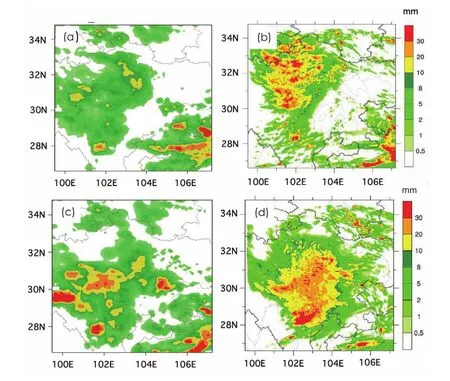
Fig.2.The 6-h accumulated precipitation(units:mm)according to the(a,c)observations and(b,d)simulation data from(a,b)0600–1200 UTC and(c,d)1200–1800 UTC 17 August 2014 in domain 1.

3.1.Fourier analysis

Fourier analysis is one of the most important methods for diagnosing wave characteristics in the atmosphere(e.g.Wheeler and Kiladis,1999;Lane and Zhang,2011;Zhang et al.,2001).To examine the spatial and temporal structures of the vertical velocity over the Sichuan area,a twodimensional Fourier analysis was applied.The Fourier analysis transformed the spatiotemporal field into a wavenumber-frequency field with a horizontal grid point interval of 10 min.By calculating the power spectra at different levels,an apparent asymmetric unimodal narrow spectrum at 10–14 km was revealed;thus,waves appeared over the Sichuan area during the precipitation process.Figure 5 shows the power spectrum of the vertical velocity at a height of 12 km along 31.1°N.Two striking domains with high power values were observed during the rainstorms.One maximum was located in the low-frequency wavenumber area,and this observation is similar to those of Wheeler and Kiladis(1999)and Lane and Zhang(2011).The other maximum was observed in a region with a frequency(ω)of 0.0083–0.0125 min−1(period of 80–120 min)and wavenumber(k)of 0.0133–0.0267 km−1(wavelength of 37.5–75 km).The positive wavenumber corresponds to an eastward-propagating wave signal,and the negative wavenumber corresponds to a westward-propagating wave signal.The peaks follow the lines in the frequency-wavenumber space that correspond to ω/k=10–25 m s−1,indicating that waves with different zonal scales and different temporal scales propagated eastward at a mean speed of 15–20 m s−1.

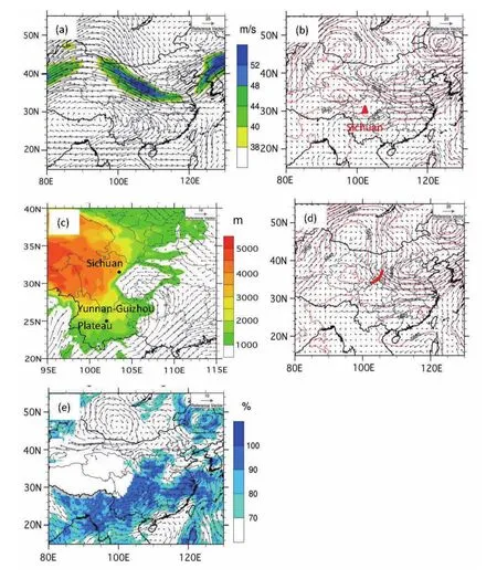
Fig.3.The distributions of(a)wind vectors(units:m s−1)and the upper-level jet(shaded;units:m s−1)at 200 hPa at 0000 UTC 17 August,(b)geopotential heights at 500 hPa(red line;units:gpm)and wind vectors(units:m s−1)at 0000 UTC 17 August,(c)wind vectors(units:m s−1)at 850 hPa and topography(shaded;units:m)at 0000 UTC 17 August,(d)geopotential heights at 500 hPa(red line;units:gpm)and wind vectors(units:m s−1)at 1200 UTC 17 August,and(e)relative humidity(shaded)and wind vectors(units:m s−1)at 700 hPa at 0000 UTC 17 August.

The spectral analysis was performed in consecutive 4-h intervals from 0000 UTC 17 to 1200 UTC 18 August,with a 2-h overlap between neighboring intervals.The lower frequency range(below0.0042min−1)was about4h,which was the same with 4-h intervals,meaning this lower frequency range was the average field.In addition,there were different scale waves that existed simultaneously in the atmosphere,but we were only concerned with the scale that had a close relationship with mesoscale systems.Thus,we chose 4 h as the interval.Therefore,signals in the lower frequency range(below 0.0042 min−1)could be omitted,because they represented the average field.

From the above analysis,prominent waves were observed at heights of 10–14 km,with a period of 80–120 min and wavelength of 37.5–75 km,during the precipitation event.The major waves propagated eastward at an average speed of 15–20 m s−1.Notably,Wang et al.(2004,2005)reported the speed of eastward-moving precipitation over the eastern Tibetan Plateau to be approximately 10–25 m s−1,which is very similar to the speed of wave propagation determined in the present study.

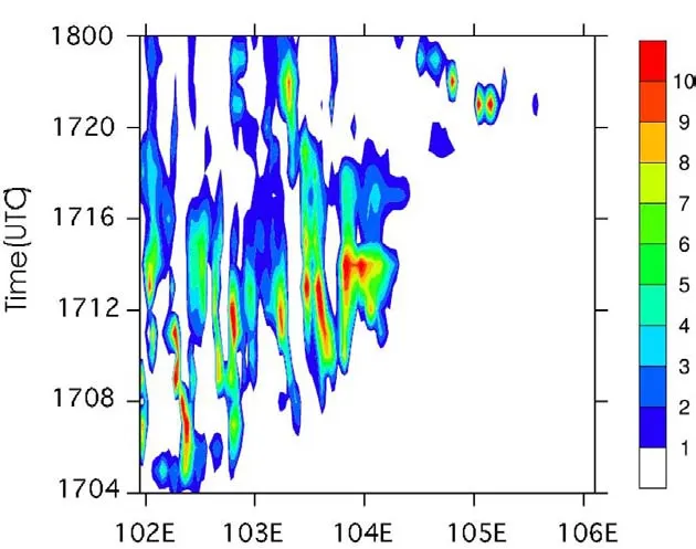
Fig.4.Temporal evolution of the 6-km total cloud mixing ratio(units:kg kg−1)(cloud water plus ice)in the simulation.

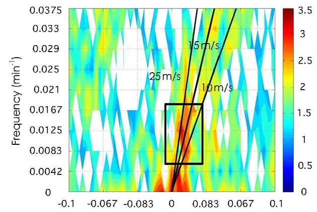
Fig.5.Power spectrum of 12-km vertical velocity along 31.1°N(red line in Fig.1a).The solid lines depict ω/k=10 m s−1,15 m s−1and 25 m s−1.

3.2.Cross-spectrum analysis

The previous subsection shows that significant spectral peaks existed in the wavenumber-frequency domain,meaning there were prominent waves occurring during the precipitation event.However,whether these waves were inertiagravity waves needed to be further verified.

Lu et al.(2005a,b)and Gao et al.(2015)noted that polarization,i.e.,when the directions of wave propagation and wave oscillation are perpendicular,is a representative characteristic of inertia-gravity waves.The phase difference between the perturbation divergence and vorticity of π/2 is an important characteristic of inertia-gravity waves.This phase shift feature is crucial for extracting the inertia-gravity waves from simulations and observational data.

On the basis of elementary equations of 3-D inertiagravity waves and their dispersion relations,we can derive the polarization relations as(Gao et al.,2015)

Where,u′,v′andw′are disturbance velocity in horizontal and vertical direction;fis Coriolis parameter;nis vertical wave number,and ω is frequency.It can be seen that the different phase shift between the divergence(D)and the vertical velocity(δ)ismπ+π/2,and the different phase shift between vertical vorticity and vertical velocity ismπ.

Then,

Based on complex variables functions theory,iis equal to π/2.When waves propagated eastward(ω >0),the vertical vorticity was located one-quarter of a wavelength(π/2)behind the divergence.When waves propagated westward(ω<0),the vertical vorticity was located one-quarter of a wavelength(π/2)before the divergence,or 3π/2 behind the divergence.Most of the time,however,±π/2 is used as the simple criterion for a different phase shift.

Based on the polarization theory mentioned above,the π/2 phase difference between the vertical vorticity and horizontal divergence is an important method for extracting inertia-gravity waves.This approach was therefore adopted in the present study,and the extracted waves were then studied via cross-spectrum analysis,as reported in this section.Figure 6 shows the square coherency and cross-phase spectra of the vorticity and divergence at 1200 UTC 17 August.Waves with distinct wavenumbers of 0.02–0.023,0.04 and 0.066 km−1(corresponding to wavelengths of 50 km,25 km and 15 km,respectively)were selected because they each displayed high coherency and phase differences of approximately π/2.In terms of the abovementioned extent of the maximum power spectra with a wavenumber of 0.0133–0.0267 km−1,the high-energy wavenumber of 0.02–0.023 km−1(wavelength of 40–50 km)was selected.Thus,the inertia-gravity waves with wavelengths of approximately 40–50 km were considered the primary waves during the precipitation period.In addition to the waves with wavenumbers of 0.02–0.023 km−1,other inertia-gravity waves with various wavenumbers and frequencies were observed;however,their energies were relatively low and less influential in the rainstorm process.

3.3.Wavelet cross-spectrum analysis

In contrast to traditional cross-spectrum analysis,which transforms signals based on the Fourier method,wavelet cross-spectrum analysis is a multiplication between a physical quantity and its conjugate based on continuous wavelet transforms(Torrence and Compo,1998;Lee,2002).The wavelet cross-spectrum method can be used to determine the time and location of inertia-gravity waves and aid in studying the development and evolution of inertia-gravity waves.

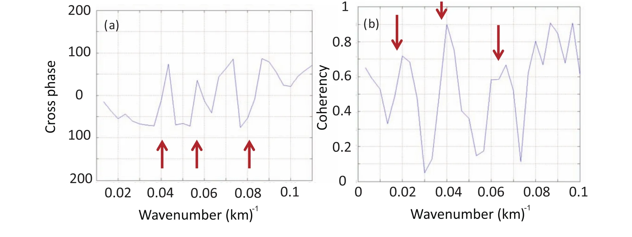
Fig.6.Cross-spectra of the 12-km vertical vorticity and divergence at 1200 UTC 17 August:(a)the phase difference between the vertical vorticity and divergence,and(b)the transformed coherency between the vertical vorticity and divergence.The arrows emphasize the significant peaks discussed in the text.

The spatial variations in the squared amplitude,coherency and phase spectra of the waves with a wavenumber of 0.025 km−1(wavelength of 40 km)were computed from the wavelet cross-spectra for the 12-km vertical vorticity and horizontal divergence(Fig.7).The Gaussian wave was chosen as the basic wave.At 1200 UTC(Figs.7a and b),a wide and stable spatial range(102.9°–103.8°E)with a phase difference of approximately π/2 and a strong coherency near 1 was observed.Also,the waves corresponded to the maximum amplitude in Fig.7c,indicating their strong wave energy.Therefore,a notable inertia-gravity wave was generated at 102.9°–103.8°E over the mountains.Similar to the results at 1200 UTC,significant inertia-gravity wave characteristics were again observed at 1300 UTC at 102.9°–103.8°E(Figs.7d–f).Notably,when the inertia-gravity waves occurred,a clear increase in precipitation was observed corresponding to the waves(Figs.7a and d).

Through spatial analysis of the wavelet cross-spectra,the key wavenumber of the inertia-gravity waves was selected.The same method was used to determine the frequency characteristic by analyzing the time dimension.The temporal variations in the squared amplitude,coherency and phase with a frequency of 0.01 min−1computed from the wavelet cross-spectra are shown in Fig.8.The spectral pro files at(31.1°N,103°E)and(31.1°N,103.7°E)in the range of the 102.9°–103.8°E(the area of inertia-gravity wave formation)were chosen.One position was located at a mountain peak,while the other was on the leeward slope of the mountain.The horizontal axis is the time dimension(from 0000 UTC 17 August to 1200 UTC 18 August).Figures 8a,b and c show that long-lived inertia-gravity waves generated from approximately 1000 UTC to 2000 UTC with a phase difference of π/2,a strong coherency,and extremely large amplitudes.At another location(31.1°N,103.7°E),prominent inertia-gravity waves were observed again at approximately 1000–1600UTC(Figs.8d–f).Thus,the inertia-gravity waves with a period of 100 min(frequency of 0.01 min−1)generated from approximately 1100 UTC to 1600 UTC during the heavy rainstorm.In addition,the peak of the 30-min accumulated precipitation occurred while the inertia-gravity waves were apparent,indicating a close relationship between the inertia-gravity waves and precipitation.Stobie et al.(1983)observed a similar result and noted that the rapid amplification of the inertia-gravity waves and the growth of convection occurred simultaneously several hours after the waves were first detected.

From the above results,we can conclude that inertiagravity waves were generated at 10–14 km,with period of 100 min and wavelength of 40–50 km.The waves propagated eastward at an average speed of 15–20 m s−1,and lasted for approximately 5 h.These waves mainly generated at 102.9°–103.8°E over the mountain.Lane and Zhang(2011)calculated the convective cloud spectra and demonstrated a similar gravity wave speed of 13ms−1.Tulich et al.(2007)presented a“slow”model of gravity waves with a speed of16–18ms−1.Thus,we believe our result to be reasonable.

3.4.Reconstruction of gravity waves

The inertia-gravity waves were filtered by extracting the frequencies of 0.01–0.0125 min−1and the wavenumbers of 0.02–0.025 km−1via the inverse Fourier transform method.The filtered field from the aggregation of the different levels constituted the reconstruction of the inertia-gravity waves.These wavenumber and frequency ranges were chosen from the results of the Fourier analysis and cross-spectrum analysis discussed above.The reconstructed inertia-gravity waves are displayed in Figs.9a and b,which show the primary fluctuations in the inertia-gravity waves during the heavy rainstorm.From1100–1200UTC(Fig.9a),the vertical velocities with negative and positive distributions were mainly located at heights of 10–14 km above the mountain peaks,and moved eastward over time.Thus,these inertia-gravity waves were very likely to be generated continuously above the mountain peak.Following this development(Fig.9b),the inertia-gravity waves were significantly enhanced and propagated farther away,being mainly located at 102.9°–104.55°E.

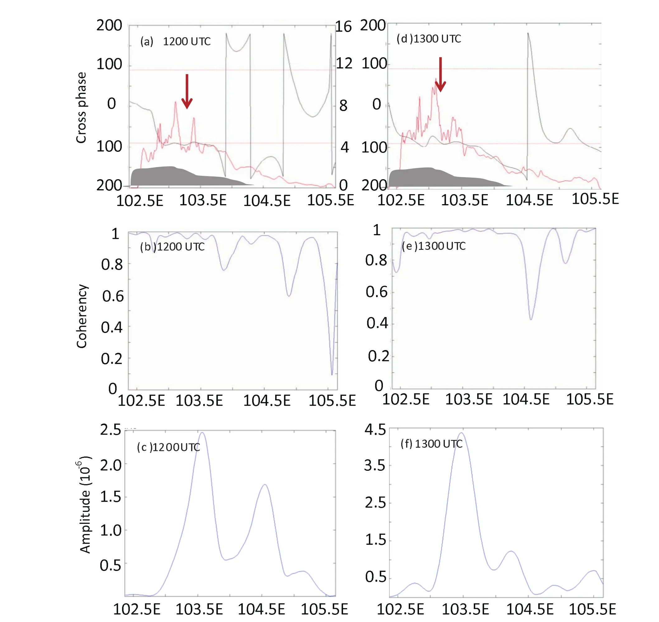
Fig.7.Wavelet cross-spectra corresponding to the horizontal wavenumber of the12-km vertical vorticity and divergence at(a–c)1200 UTC and(d–f)1300 UTC 17 August:(a,d)the phase difference(black line)and 30-min accumulated precipitation(red line;units:mm);(b,e)the transformed coherency;and(c,f)the cross amplitude.The arrows emphasize the significant peaks discussed in the text.The gray region denotes the topography.

Figures 9c and d show the vertical profiles of vertical velocity,wind vectors,the high-level jet,and 30-min accumulated precipitation along 31.1°N.Strong and stable westerly flow was observed in the upper levels during the precipitation event.The peak precipitation occurred on the leeward(eastern)slope of the mountain.At 1200 UTC(Fig.9c),a wide range of upward motion appeared over the windward slope of the mountain and over the mountain peaks due to orographic uplift.Then,after the westerly wind moved over the mountain,there were fluctuations generated in the air flow,leading to negative and positive changes that reflected the generation of eastward-propagating inertia-gravity waves.When the eastward-propagating waves approached the entrance of the high-level jet,the waves were enhanced due to the nongeostrophic balance.With the increase in vertical motion,the inertia-gravity waves gradually became enhanced,and the corresponding surface precipitation increased.At 1400 UTC(Fig.9d),the strength of the inertia-gravity waves and the accumulated precipitation reached near-simultaneous peaks.As the coupled effects of orographic uplift and the high-level jet disintegrated,the inertia-gravity waves weakened and gradually died out.

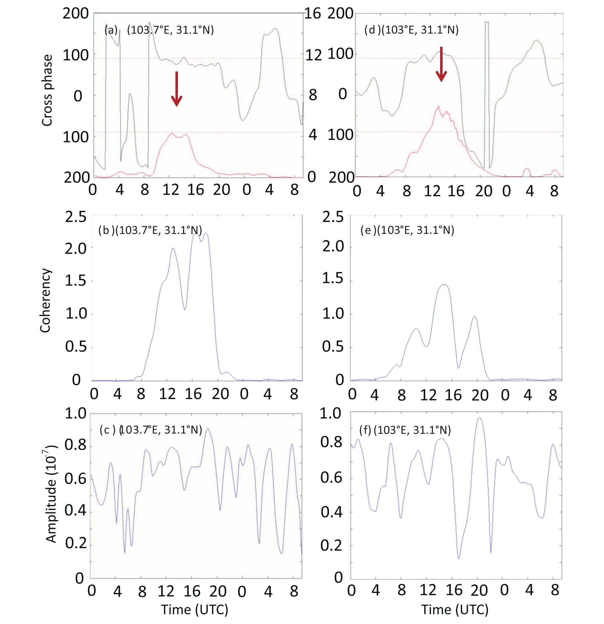
Fig.8.As in Fig.7 but for frequency.

Figure 10 displays the time–longitude distributions of the reconstructed inertia-gravity waves and 60-min accumulated precipitation. Eastward-moving inertia-gravity waves occurred from1100 UTC to 1700 UTC within102.9°–104.55°E over the mountain(Fig.10a).Figure 10b shows that accumulated precipitation was highest primarily within 102.9°–103.5°E and generated from 1100 UTC to 1600 UTC,which corresponded well with the period of enhanced inertia-gravity waves.Many researchers(e.g.,Uccellini,1975;Koch and Siedlarz,1999;Lane and Zhang,2011)have examined the interaction between inertia-gravity waves and deep convection and proposed that mesoscale gravity waves can cause convective instability and initiate thunderstorm development;in turn,the latent heat release feeds back to the background waves,triggering or amplifying the gravity waves.

3.5.Intrinsic wave characteristics

Aside from showing wave patterns,quantifying the intrinsic wave characteristics,such as the intrinsic frequency,intrinsic speed or vertical wavelengths,is also very important for a thorough understanding of such waves.

The dispersion relation for inertia-gravity waves was taken to be(Kitchen and McIntyre,1980)

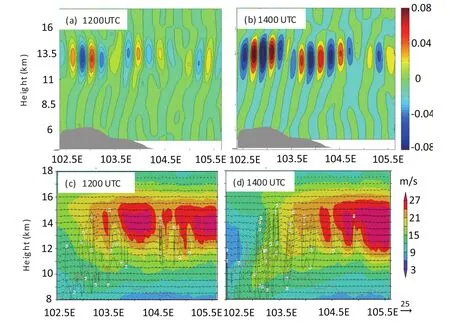
Fig.9.(a,b)Reconstructed eastward-propagating inertia-gravity waves(frequency of 0.001–0.0125 min−1,wavenumber of 0.02–0.025 km−1)with oscillations in the vertical velocity(units:m s−1)and(c,d)vertical pro files of the positive vertical velocity(contours;units:m s−1),wind vector(vectors;units:m s−1),high-level jet(shaded units:m s−1)and 30-min accumulated precipitation(red line;units:mm)at(a,c)1200 UTC and(b,d)1400 UTC 17 August.The gray region denotes the topography.

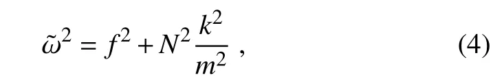
The average frequency ω,obtained in Fig.5,was about 2×10−4s−1,and the average horizontal wavenumberkwas about 2.22×10−5m−1(maximum value in Fig.5).The average background flow at heights of 10–14 km was about 15 m s−1,as obtained in Fig.12b.According to the above formula,the intrinsic frequencywas about 1.3×10−4s−1.Substitutinginto the dispersion relation for inertia-gravity waves yielded the vertical wavenumberm.Finally,the vertical wavenumber was approximately 1.1×10−3m−1,and thus the vertical wavelength was about 1 km.The ratio of the horizontal wavelength to the vertical wavelength was 50:1,and thus these waves mainly propagated horizontally and far away(Bian et al.,2005).

3.6.Ducting of the gravity waves

The reconstruction of the inertia-gravity waves provides information about their generation,propagation,and location during the precipitation event.This section discusses the favorable conditions for the propagation of inertia-gravity waves.

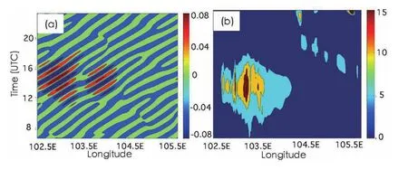
Fig.10.Time–longitude distribution of(a)the reconstructed inertia-gravity waves with oscillations in the vertical velocity(units:m s−1)at 13 km,and(b)the 60-min accumulated precipitation(units:mm)from 0700 UTC to 2400 UTC 17 August.

Gravity waves in the atmosphere can propagate freely in the vertical direction and tend to lose their energy through vertical propagation before traveling even a single wavelength horizontally.Thus,gravity wave ducting is needed.Lindzen and Tung(1976)analyzed this phenomenon and concluded that the favorable conditions for ducted inertiagravity waves include effective ducting and critical levels.Ducting is a statically stable(or conditionally stable)and sufficiently thick stratification,topped by a stable reflecting layer.A stable reflector consists of a shear unstable layer with a Richardson number<0.25(including negative values).The reflectivity is greatly enhanced if the conditionally unstable layer contains a critical level where the flow speed in the environment equals the phase-speed of the waves.In the over-reflection layer,the waves can extract energy from the mean flow at the critical level,which significantly affects the lifetime of a wave.Thus,the ducting and critical level conditions of the atmosphere have significant influence on inertiagravity wave propagation.

Figure 11 illustrates the vertical pro file of the Richardson number,u-wind(zonal wind)of approximately 20 m s−1and vertical shear of theu-wind along 31.1°N.Layers with Richardson numbers smaller than 0.25 at heights of 10–14 km are illustrated in Fig.11a.These layers served as shear unstable layers for ducting.In addition,layers withu-wind speeds of 20 m s−1were embedded in the reflectivity layers.This speed was similar to the phase speed of the inertia-gravity waves,reflecting the existence of a critical level.Such layers tend to trap vertically propagating inertia-gravity waves and enable waves to extract energy from the background flow.Lindzen and Tung(1976)noted that in the absence of shear,the long lifetimes of the observed mesoscale waves cannot be explained.Thus,Fig.11b shows the strong vertical wind shear above and below the ducting zone,which was mainly due to a high-level jet.These shear areas can greatly enhance the reflections.These favorable thermal and dynamic conditions effectively trapped the inertia-gravity waves from propagating horizontally and prevented a significant loss of energy,thus maintaining the longlived waves.In the above analysis(Fig.9),the inertia-gravity waves propagated upward in the regions of 102.5°–103.3°E and 103.7°–104.5°E,and downward in the region of 103.3°–103.7°E,which demonstrated the reflection phenomenon.

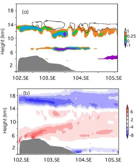
Fig.11.Vertical pro file of(a)the Richardson number(shaded)and the wind speed of U ≈ 20 m s−1(contours),and(b)vertical shear of the u-wind(shaded units:s−1)at 1130 UTC 17 August.The gray region denotes the topography.

In addition,the wave trapping discussed by Yang and Houze(1995)and Fovell et al.(2006)can be explained by the Scorer parameterl2(Scorer,1949;Crook,1988).The Scorer parameter is a good indicator of wave reflection and can be approximated as follows:

whereN2is the sub-saturated Brunt–Väisälä frequency,Uzzis second derivative of¯u,andcis the phase speed of the inertia-gravity waves,which is approximately 20 m s−1.A sudden decrease inl2with height indicates that some of the vertically propagating waves will be trapped.

Figure 12 presents the vertical pro files ofN2,Uandl2.A sudden decrease inl2was observed at approximately 14 km(Fig.12c).This variation likely reflects an effective ducting for the inertia-gravity waves.The greatly reduced stability(Fig.12a)and large negative curvature of wind shear(Fig.12b)led to a sudden decrease inl2values.

4.Additional simulations

4.1.Orographic simulations

The above analysis shows that the terrain was an important reason for triggering the inertia-gravity waves during a rainstorm event.In this section,some numerical sensitivity experiments are conducted to examine the effects of different terrain scales on the generation and evolution of inertiagravity waves.

To examine the sensitivity of the generation and propagation of inertia-gravity waves to the terrain,simulations were rerun using different scales of terrain with all other aspects of the simulation unchanged.Here,the method of wavelet analysis is used to decompose the terrain into diあerent scales details of the experiment design are given in Table 1.

The new terrain filtering the disturbance smaller than 8km in the S1 experiment is shown in Fig.13a.Compared with theinitial terrain,the primary difference was that the small terrain disturbances at the top of the mountain were smoothed(near 103°N).The distribution of the power spectrum in the S1 experiment was similar to that in the control(CTL)experiment( figure omitted);thus,the small terrain disturbances had little effect on the period and wavelength of the inertiagravity waves.However,the generation of the inertia-gravity waves occurred at approximately 1400 UTC in the S1 experiment,which was much later than that in the CTL experiment(Fig.10b).Therefore,the small terrain disturbance at the top of the mountain was conducive to trigger the inertia-gravity waves.At the same time,the occurrence of heavy precipitation was delayed( figure omitted),which is likely due to the delay of the inertia-gravity waves.

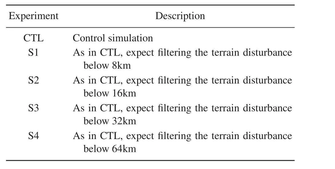
Table 1.Summary of the experiment design.

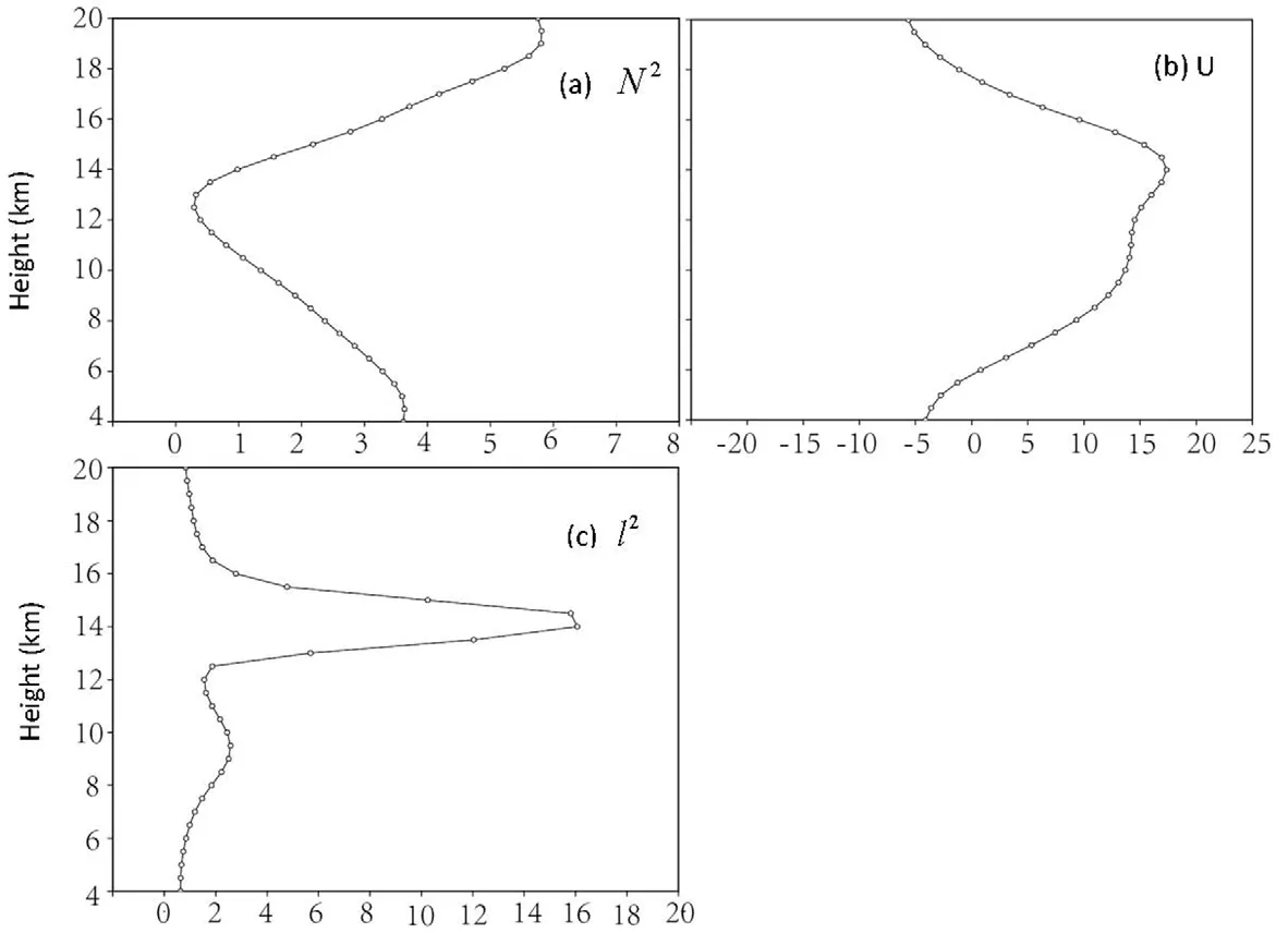
Fig.12.Area-averaged pro files of the(a)Brunt–Väisälä frequency N2(units:10−4s−2),(b)u-component of wind speed(units:m s−1)and(c)Scorer parameter l2(units:10−5m−2)at 1030 UTC 17 August.

Fig.13.The(a,c,e,g)vertical pro files of the topography(units:m)in experiments S1,S2,S3,and S4,(b)time–longitude distribution of the reconstructed inertia-gravity waves with oscillations in the vertical velocity(units:m s−1),and(d,f,g)power spectra of the 12-km vertical velocity along 31.1°N for experiments S2,S3,and S4.

Figure 13c and 13e show the new terrain filtering the disturbance smaller than 16 km and 32 km in the S2 and S3 experiment,respectively.Compared with the initial terrain,the new terrains were smoothed and lacked small terrain disturbances.The terrain in S2 was narrower than that in the CTL experiment,and the terrain in S3 was wider than that in the CTL experiment.The power spectrum in the S2 experiment showed that the spectral peaks in the wavenumber-frequency domain occurred in the frequency range of 0.0083-0.0125 min−1,which was larger than that in the CTL experiment(Fig.13d).And the power spectrum in the S3 experiment showed that the spectral peaks occurred in the frequency range of 0.0042–0.0083 min−1,which was smaller than that in the CTL experiment(Fig.13f).The results from the comparison between the S2 and S3 experiments suggested that different terrain scales significantly influenced the characteristics of the inertia-gravity waves.The frequency and wavenumber of the inertia-gravity waves generated by the large mountain range were relatively small,and those generated by the small mountain range were relatively large.

The terrain filtering the disturbance smaller than 64km in the S4 experiment is shown in Fig.13g.Notably,the new terrain was not only smoothed but also lower than the initial terrain.Meanwhile,the slope of the east side of the mountain was reduced,and the lifting effect of the terrain was weakened.Eastward-propagating waves were observed at height of 12 km,but the wave energy was much weaker than that in the CTL experiment and was mostly concentrated in largescale and mean fields.Meanwhile,the accumulated precipitation was much lower than that observed in the CTL experiment,which is likely due to the weakened inertia-gravity waves.

It needs to be noticed that the high-frequency and largewavenumber wave components illustrated in Figs.13d,f,and h maybe false waves and can be neglected.Because the waves occurred at top-right of these figures,corresponding to about time period of 20 min,while the simulated result export every ten minutes.The temporal resolution of pattern result is relatively too low to small scale wave with 20 min.

Therefore,the results of the sensitivity experiments show that the different terrain scales significantly influenced the generation and propagation of inertia-gravity waves.The small terrain disturbance at the top of the mountain was conducive to triggering the inertia-gravity waves.In addition,the orographic scales significantly affected the characteristics of the inertia-gravity waves.The frequency and wave-number of the waves generated by the large mountain range were relatively small,and those generated by the small mountain range were relatively large.

4.2.Diabatic simulations

In addition to the role of terrain, the force of diabatic heating also plays an important role in the generation and propagation of the inertia-gravity waves.However,which one(terrain or diabatic heating)was the key reason for inertia-gravity waves’evolution?Here,we perform another simulation,in which diabatic heating is turned off,to examining the effect of diabatic heating.

The power spectrum and the reconstructed inertia-gravity waves were shown in Fig 14.There was one high power values occurred in Fig 14a,which primarily located in a region with frequency of 0.0042–0.0083 min−1and wavenumber of 0.0133–0.0267 km−1.Compared with Fig 5,the waves generated in diabatic simulation have longer periods and similar wavelengths.What is interesting is that turning off the diabatic heating process,the strength of reconstructed inertiagravity waves was much weaker,especially the waves located at approximately 104°E(Fig 14 b,c).In additions,there was no obvious fractured wave activities occurred.Therefore,the comparison shows that the diabatic heating force had significant impact on the inertia-gravity wave propagation.Turning off the diabatic heating,the frequency of waves had been changed and the strength of waves became weakened,but the inertia-gravity waves can still be observed. Thus it can be concluded that the orographic effect played the key role in generating the inertia-gravity waves occurred in this rainstorm,and the moist convection enhance the waves and benefited the long-lived waves.

5.Conclusions and discussion

In this study,a numerical experiment was performed using the WRF model to simulate an orographic rainstorm that occurred on 17 August 2014.The generation and propagation of inertia-gravity waves during the precipitation event were analyzed.

To examine the spatial and temporal structures of the inertia-gravity waves and identify the wave types,three wave-number-frequency spectral analysis methods,including Fourier analysis,cross-spectral analysis and wavelet crossspectral analysis,were applied.First,Fourier analysis was performed to extract the characteristics of the critical-scale waves during the precipitation event.Then,considering the polarization relationship,cross-spectral analysis and wavelet cross-spectral analysis were used to demonstrate that the critical-scale waves were inertia-gravity waves.Through this method,the inertia-gravity waves with period of 80–100 min and wavelength of 40–50 km at heights of 10–14 km were extracted from the atmosphere. The predominant inertia-gravity waves propagated eastward at an average speed of 15–20 m s−1,from 1100 UTC to 1600 UTC,and they were located predominantly at 102.9°–104°E over the mountain.The advantage of wavelet cross-spectral analysis is that it not only reflects the spectral characteristics of the waves but also locates the temporal and spatial distribution of inertia-gravity waves.

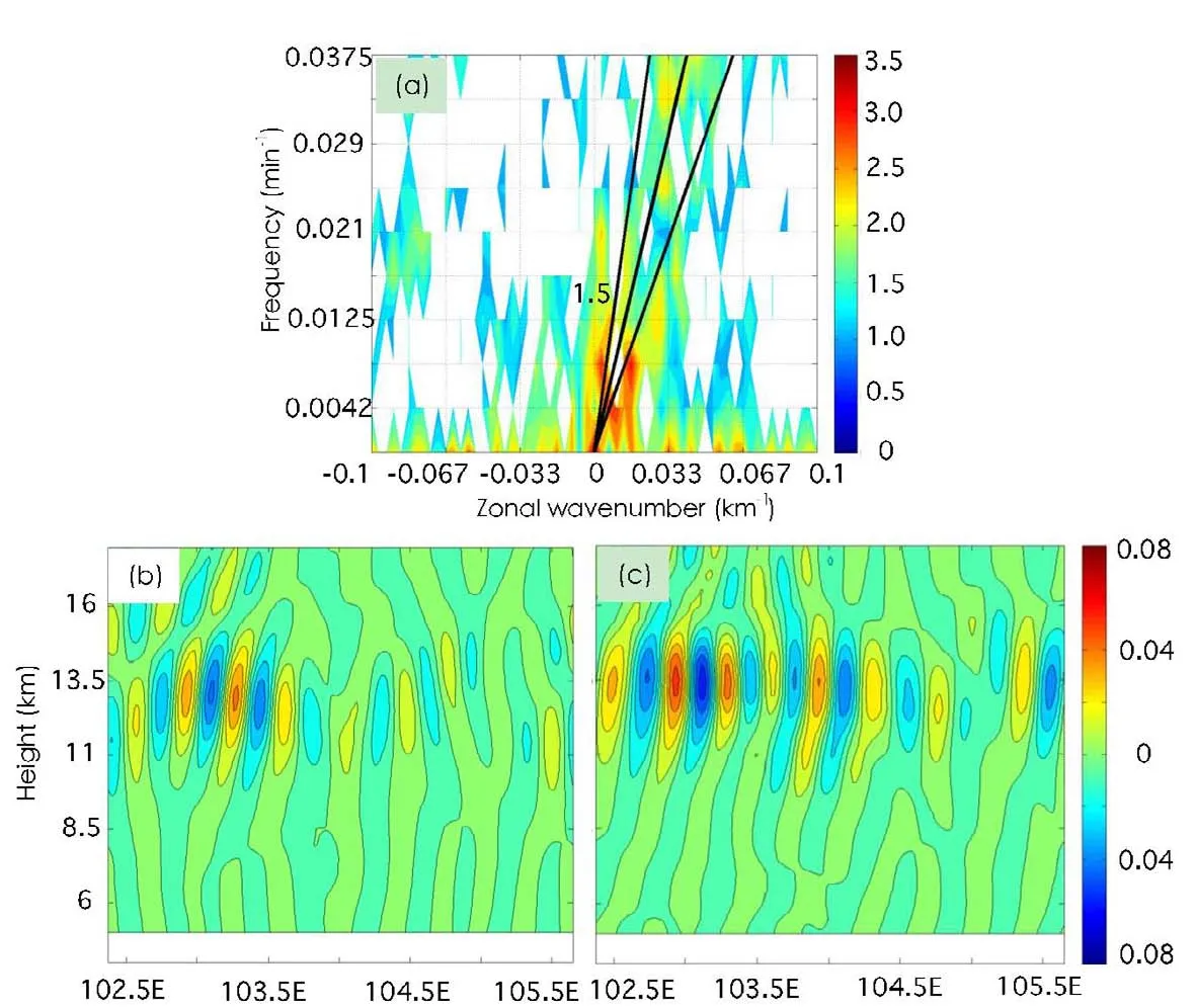
Fig.14.(a)Power spectrum of 12-km vertical velocity along 31.1°N.(b,c)Reconstructed eastward-propagating inertiagravity waves with oscillations in the vertical velocity(units:m s−1).

Based on inverse Fourier transform,the reconstructed inertia-gravity waves were shown intuitively to provide a better physical understanding of these waves.Notably,the comparison between the reconstructed inertia-gravity waves and accumulated precipitation shows that there was positive feedback between the inertia-gravity waves and precipitation.Many researchers(e.g.Uccellini,1975;Koch and Siedlarz,1999;Lane and Zhang,2011)have examined the interaction between inertia-gravity waves and deep convection and proposed that mesoscale gravity waves were capable of causing convective instability and initiating thunderstorm development;in turn,the latent heat release provided feedback to the background waves,triggering or amplifying the gravity waves.Then,the Richardson number and Scorer parameter were used to demonstrate that the eastward-moving inertiagravity waves were trapped in an effective ducting zone with strong reflector and critical level conditions,which were the primary mechanisms that led long-lived inertia-gravity waves.

Finally,some numerical sensitivity experiments were conducted to examine the effects of different terrain scales and the diatatic heating on inertia-gravity waves.The results show that the different terrain scales significantly influenced the generation and propagation of inertia-gravity waves.The small terrain disturbance at the top of the mountain was conducive to triggering the inertia-gravity waves.In addition,the frequency and wave-number of the inertia-gravity waves generated by the large mountain range were relatively small,and those generated by the small mountain range were relatively large.The diabatic simulations show that the orographic effect played the key role in generating the inertiagravity waves occurred in this rainstorm,and the moist convection enhance the waves and benefit the long-lived waves.

This study summarizes the basic characteristic of inertiagravity waves during an orographic precipitation that occurred in the Sichuan area.However,the universality of the characteristics of inertia-gravity waves in the Sichuan area should be verified with additional cases.In this paper,the results of wavelet cross-spectral analysis and inverse Fourier transform show that positive feedback occurred between the inertia-gravity waves and precipitation.However,further studies are needed in the future to determine the in-depth feedback mechanisms and relationships.

Acknowledgements.We thank Y.C.ZHANG for the valuable discussion.The GFS data used in this paper are available at http://nomads.ncdc.noaa.gov/data/gfs4.This study was supported by Study on Key Techniques of convective gale monitoring and forecasting in spring in Southern China(GYHY201406002),the National Natural Science Foundation of China(41705027,41775140,41175060,91437215,and 41575047),the research project of Heavy Rain and Drought-Flood Disasters in Plateau and Basin Key Laboratory of Sichuan Province(SZKT2016002)and Open projects of Plateau Atmosphere and Environment Key Laboratory of Sichuan Province(PAEKL-2015-K2).

Alexander,M.J.,and L.Pfister,1995:Gravity wave momentum flux in the lower stratosphere over convection.Geophys.Res.Lett.,22,2029–2032,https://doi.org/10.1029/95GL01984.

Bian,J.C.,H.B.Chen,and D.R.Lv,2005:Statistics of gravity waves in the lower stratosphere over Beijing based on high vertical resolution radiosonde.Science in China Series D:Earth Sciences,48,1548–1558,https://doi.org/10.1360/03yd0512.

Chen,D.,Z.Y.Chen,and D.R.Lv,2013:Spatiotemporal spectrum and momentum flux of the stratospheric gravity waves generated by a typhoon.Science China:Earth Sciences,56,54–62,https://doi.org/10.1007/s11430-012-4502-4.

Crook,N.A.,1988:Trapping of low-level internal gravity waves.J.Atmos.Sci.,45,1533–1541,https://doi.org/10.1175/1520-0469(1988)045<1533:TOLLIG>2.0.CO;2.

Doswell III,C.A.,H.E.Brooks,and R.A.Maddox,1996:Flash flood forecasting:An ingredients-based methodology.Wea.Forecasting,11,560–581,https://doi.org/10.1175/1520-0434(1996)011<0560:FFFAIB>2.0.CO;2.

Fovell,R.G.,G.L.Mullendore,and S.H.Kim,2006:Discrete propagation in numerically simulated nocturnal squall lines.Mon.Wea.Rev.,134,3735–3752,https://doi.org/10.1175/MWR3268.1.

Fritts,D.C.,and M.J.Alexander,2003:Gravity wave dynamics and effects in the middle atmosphere.Rev.Geophys.,41,1003,https://doi.org/10.1029/2001RG000106.

Gamage,N.,and W.Blumen,1993:Comparative analysis of lowlevel cold fronts:Wavelet,Fourier,and empirical orthogonal function decompositions.Mon.Wea.Rev.,121,2867–2878, https://doi.org/10.1175/1520-0493(1993)121<2867:CAOLLC>2.0.CO;2.

Gao,S.T.,L.K.Ran,and X.F.Li,2015:The Mesoscale Dynamic Meteorology and Its Prediction Method.Meteorological Press.(in Chinese)

Grivet-Talocia,S.,F.Einaudi,W.L.Clark,R.D.Dennett,G.D.Nastrom,and T.E.VanZandt,1999:A 4-yr climatology of pressure disturbances using a barometer network in central Illinois.Mon.Wea.Rev.,127,1613–1629,https://doi.org/10.1175/1520-0493(1999)127<1613:AYCOPD>2.0.CO;2.

Janji´c,Z.I.,1994:The step-mountain eta coordinate model:Further developments of the convection,viscous sublayer,and turbulence closure schemes.Mon.Wea.Rev.,122,927–945,https://doi.org/10.1175/1520-0493(1994)122<0927:TSMECM>2.0.CO;2.

Jewett B.F.,M.K.Ramamurthy,and R.M.Rauber,2003:Origin,evolution,and finescale structure of the St.Valentine’s day mesoscale gravity wave observed during STORM-FEST.Part III:Gravity wave genesis and the role of evaporation.Mon.Wea.Rev.,131,617–633,https://doi.org/10.1175/1520-0493(2003)131<0617:OEAFSO>2.0.CO;2.

Kim,Y.J.,S.D.Eckermann,and H.Y.Chun,2003:An overview of the past,present and future of gravity-wave drag parametrization for numerical climate and weather prediction models.Atmos.Ocean,41,65–98,https://doi.org/10.3137/ao.410105.

Kitchen,E.H.,and M.E.McIntyre,1980:On whether inertiogravity waves are absorbed or reflected when their intrinsic frequency is Doppler-Shifted towards.J.Meteor.Soc.Japan,58,118–126,https://doi.org/10.2151/jmsj1965.58.2118.

Koch,S.E.,and L.M.Siedlarz,1999:Mesoscale gravity waves and their environment in the central united states during STORM-FEST.Mon.Wea.Rev.,127,2854–2879,https://doi.org/10.1175/1520-0493(1999)127<2854:MGWATE>2.0.CO;2.

Lane,P.T.,and M.W.Moncrieff,2008:Stratospheric gravity waves generated by multiscale tropical convection.J.Atmos.Sci.,65,2598–2614,.

Lane,T.P.,and F.Q.Zhang,2011:Coupling between gravity waves and tropical convection at mesoscales.J.Atmos.Sci.,68,2582–2598,https://doi.org/10.1175/2011JAS3577.1.

Lee,D.,2002:Analysis of phase-locked oscillations in multichannel single-unit spike activity with wavelet crossspectrum.Journal of Neuroscience Methods,115,67–75,https://doi.org/10.1016/S0165-0270(02)00002-X.

Li,M.C.,1978:Studies on the gravity wave initiation of the excessively heavy rainfall.Scientia Atmospherica Sinica,2,201–209,https://doi.org/10.3878/j.issn.1006-9895.1978.03.03.(in Chinese with English abstract)

Lindzen,R.S.,and K.K.Tung,1976:Banded convective activity and ducted gravity waves.Mon.Wea.Rev.,104,1602–1617, https://doi.org/10.1175/1520-0493(1976)104<1602:BCAADG>2.0.CO;2.

Lu,C.G.,S.E.Koch,and N.Wang,2005a:Stokes parameter analysis of a packet of turbulence-generating gravity waves.J.Geophys.Res.,110,D20105,https://doi.org/10.1029/2004 JD005736.

Lu,C.G.,S.Koch,and N.Wang,2005b:Determination of temporal and spatial characteristics of atmospheric gravity waves combining cross-spectral analysis and wavelet transformation.J.Geophys.Res.,110,D01109,https://doi.org/10.1029/2004JD004906.

McLandress,C.,M.J.Alexander,and D.L.Wu,2000:Microwave limb sounder observations of gravity waves in the stratosphere:A climatology and interpretation.J.Geophys.Res.,105,11947–11967,https://doi.org/10.1029/2000JD900097.

Mlawer,E.J.,S.J.Taubman,P.D.Brown,M.J.Iacono,and S.A.Clough,1997:Radiative transfer for inhomogeneous atmospheres:RRTM,a validated correlated-k model for the longwave.J.Geophys.Res,10,16663–16682,https://doi.org/10.1029/97JD00237.

Sato,K.,1992:Vertical wind disturbances in the afternoon of midsummer revealed by the MU radar.Geophys.Res.Lett.,19,1943–1946,https://doi.org/10.1029/92GL02244.

Scorer,R.S.,1949:Theory of waves in the lee of mountains.Quart.J.Roy.Meteor.Soc.,75,41–56,https://doi.org/10.1002/qj.49707532308.

Stobie,J.G.,F.Einaudi,and L.W.Uccellini,1983:A case study of gravity waves-convective storms interaction:9 May 1979.J.Atmos.Sci.,40,2804–2830,https://doi.org/10.1175/1520-0469(1983)040<2804:ACSOGW>2.0.CO;2.

Thompson,G.,P.R.Field,R.M.Rasmussen,and W.D.Hall,2008:Explicit forecasts of winter precipitation using an improved bulk microphysics scheme.Part II:Implementation of a new snow parameterization.Mon.Wea.Rev.,136,5095–5115,https://doi.org/10.1175/2008MWR2387.1.

Torrence,C.,and G.P.Compo,1998:A practical guide to wavelet analysis.Bull.Amer.Meteor.Soc.,79,61–78,https://doi.org/10.1175/1520-0477(1998)079<0061:APGTWA>2.0.CO;2.

Tulich,S.N.,D.A.Randall,and B.E.Mapes,2007:Vertical-mode and cloud decomposition of large-scale convectively coupled gravity waves in a two-dimensional cloud-resolving model.J.Atmos.Sci.,64,1210–1229,https://doi.org/10.1175/JAS3884.1.

Uccellini,L.W.,1975:A case study of apparent gravity wave initiation of severe convective storms.Mon.Wea.Rev.,103,497–513,https://doi.org/10.1175/1520-0493(1975)103<0497:ACSOAG>2.0.CO;2.

Vincent,R.A.,and M.J.Alexander,2000:Gravity waves in the tropical lower stratosphere:An observational study of seasonal and interannual variability.J.Geophys.Res.,105,17971–17982,https://doi.org/10.1029/2000JD900196.

Wang,C.C.,G.T.J.Chen,and R.E.Carbone,2004:A climatology of warm-season cloud patterns over east Asia based on GMS infrared brightness temperature observations.Mon.Wea.Rev.,132,1606–1629,https://doi.org/10.1175/1520-0493(2004)132<1606:ACOWCP>2.0.CO;2.

Wang,C.C.,G.T.J.Chen,and R.E.Carbone,2005:Variability of warm-season cloud episodes over east Asia based on GMS infrared brightness temperature observations.Mon.Wea.Rev.,133,1478–1500,https://doi.org/10.1175/MWR2928.1.

Wang,S.G.,and F.Q.Zhang,2007:Sensitivity of mesoscale gravity waves to the baroclinicity of jet-front systems.Mon.Wea.Rev.,135,670–688,https://doi.org/10.1175/MWR3314.1.

Wang,W.,J.Liu,and X.J.Cai,2011:Impact of mesoscale gravity waves on a heavy rainfall event in the east side of the Tibetan Plateau.Transactions of Atmospheric Sciences,34,737–747,https://doi.org/10.3969/j.issn.1674-7097.2011.06.012.(in Chinese with English abstract)

Weng,H.Y.,and K.M.Lau,1994:Wavelets,period doubling,and time-frequency localization with application to organization of convection over the tropical western Pacific.J.Atmos.Sci.,51,2523–2541,https://doi.org/10.1175/1520-0469(1994)051<2523:WPDATL>2.0.CO;2.

Wheeler,M.,and G.N.Kiladis,1999:Convectively coupled equatorial waves:Analysis of clouds and temperature in the wavenumber-frequency domain.J.Atmos.Sci.,56,374–399,https://doi.org/10.1175/1520-0469(1999)056<0374:CCEWAO>2.0.CO;2.

Wu,D.,D.H.Wang,and G.B.He,2016:Gravity wave characteristics in two summer heavy rainfall in the Qinghai-Xizang Plateau.Plateau Meteorology,35,854–864,https://doi.org/10.7522/j.issn.1000-0534.2015.00066.(in Chinese with English abstract)

Yang,M.J.,and R.A.Houze Jr.,1995:Multicell squall-line structure as a manifestation of vertically trapped gravity waves.Mon.Wea.Rev.,123,641–661,https://doi.org/10.1175/1520-0493(1995)123<0641:MSLSAA>2.0.CO;2.

Zhang,F.Q.,S.E.Koch,C.A.Davis,M.L.Kaplan,and S.E.Koch,2001:Wavelet analysis and the governing dynamics of a large-amplitude mesoscale gravity-wave event along the east coast of the united states.Quart.J.Roy.Meteor.Soc.,127,2209–2245,https://doi.org/10.1002/qj.49712757702.

Zhang,Y.C.,F.Q.Zhang,and J.H.Sun,2014:Comparison of the diurnal variations of warm-season precipitation for East Asia vs.North America downstream of the Tibetan Plateau vs.the Rocky Mountains.Atmospheric Chemistry and Physics,14,10741–10759,https://doi.org/doi:10.5194/acp-14-10741-2014.