轴流风机叶尖泄漏流动的大涡模拟

Alexej Pogorelov Matthias Meinke Wolfgang Schroder

(Institute of Aerodynamics,RWTH Aachen University,Wullnerstr.5a,52062 Aachen,Germany)

0 Introduction

The tip-gap between the blade and the casing wall has a strong impact on the performance and especially the noise generation of axial fans and turbo machines.The noise reduction has been a continuous challenge for engineers due to the intricate flow structures in the tip gap region.To predict such fan noise components,hybrid CFD-Computational Aeroacoustics(CAA)methods can be applied,which,however,need highly resolved flow data to reliably compute the noise from the unsteady turbulent sources.Reynoldsaveraged Navier-Stokes(RANS)simulations have been primarily used in the past to determine the flow field,since theyarecomputationallyefficient.Dependingontheflowfield,the RANS findings are,however,not always reliable[1-3].Especially the flow dynamics in the tip-leakage region is usually not accurately predicted due to the existence of typically unsteady vortices and strong streamline curvature,for which RANS models are known to be not reliable.

For this reason,a large-eddy simulation(LES)is used to predict the flow field which can capture the most energetic turbulent scales.Several authors have already applied LES to tip-leakage flows.Investigations have been performed,e.g.,by You et al[4-7].for a linear cascade with a moving end wall.They studied the tip-leakage flow dynamics and the effect of the tip-gap size on the vortical structures with special focus on viscous losses and low pressure fluctuations.They found that varying the tip-gap size has an effect on the formation and the trajectory of the tip-leakage vortex.Rotating effects have not been considered.Furthermore,they conclude that the detailed dynamics of the tip-leakage flow is still not understood and that the unsteady nature of the flow is beyond the prediction capability of RANS approaches[6].Boudet etal.[8]performed computations of a single airfoil tip-clearance flow focusing on the noise generation.Although the velocity fluctuations inside the boundary layer of the casing plate were underestimated,a marginal influence on the tip-clearance flow was observed in their configuration.Cahuzac et al[9].studied the tip-clearance flow in a rotor blade.They showed the good capabilities of LES to predict the broadband noise.In most of those studies,structured meshes were used,which are tedious to generate due to the complex geometry around the tip gap.

The main objective of this study is to demonstrate that a Cartesian flow solverwith fully automatic mesh generation can be efficiently used to perform highly accurate LES of flows of axial fans.Furthermore,a formulation of a periodic boundary condition in the azimuthal direction for Cartesian hierarchical meshes will be introduced which is a must for the aforementioned LES computations.

Thispaperisorganized asfollows.First,the numerical method is described.Second,the numerical setup and the boundary conditions are presented.Then,the results of a grid convergence study are presented and results are presented for two volume rates.Subsequently,theinstantaneousandtime-averagedflowfieldare discussed and compared to RANS results.Finally,the influence of the tip-gap size is investigated before some conclusions are drawn.

2 Numerical Method

2.1 Governing Equations

The numerical simulation is based on the nondimensionalized Navier-Stokes equations

The quantity QQ=[ρ，ρu，ρE]Tis the vector of the conservative variables with the densityρ,velocity vector uu,and the total specific energyE=e+ uu2/2 containing the specific energy e.A body force bb is added to the right-hand side to take into account Coriolis and centrifugal forces since the equations are solved in a rotating frame of reference.The flux tensor,which can be decomposed into an inviscidinvand a viscous partvis,and the body force bb are defined as

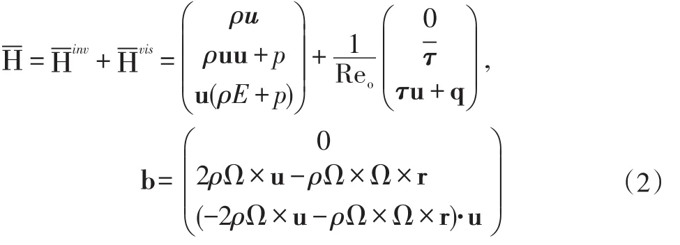
whereΩis the angular velocity vector.All variables are non-dimensionalized by fluid properties at the state of rest.That is,the Reynolds number is obtained by Re0=ρ0a0lref/η0,where a0denotes the speed of sound andlrefthe characteristic length.Furthermore,the volume viscosity is assumed to be zero such that the stress tensor for a Newtonian fluid-τcan be written as

The vector of heat conduction qq is formulated as

according to Fourier's law with the gradient of the static temperature∇T.The quantityλis the thermal conductivity,γthe ratio of specific heats.For a constant Prandtl number the thermal conductivity isλ(T)=η(T)and the dynamic viscosity is calculated using Sutherland's Law.The values forγand Pr areγ=1:4 and Pr=0:72.The system of equations is closed by the equation of state for an ideal gas.

The solver uses a modified advection upstream splitting method(AUSM[11])in a low dissipation version suitable for LES proposed by Meinke etal.[12].The equations are discretized on a locally refined Cartesian mesh,where the derivatives are approximated by a weighted least squares method.For the integration in time,a 5-stage second-order accurate Runge-Kutta scheme is used[13].The overall accuracy is second order in time and space.Details on the discretization and the computation of the inviscid and viscous surface fluxes can be found in Hartmann et al.[11].To handle sharp edges a fully conservative cut-cell method is used.Small cells on the boundaries are treated by a flux-redistribution method developed by Schneiders et al.[14]to avoid numerical instabilities.

2.2 Cartesian Mesh Generation

The hierarchical Cartesian mesh for the finite-volume solver is generated by a parallel Cartesian grid generator[10].Compared to structured boundary fitted meshes,Cartesian grids typically contain more cells,especially for high Reynolds number flow,where isotropic refinement of the mesh near walls lead to small spatial steps in all three space dimensions.The advantages of Cartesian grids are the higher accuracy due to per definition orthogonal mesh lines and the possible completely automatic and parallel grid generation on an arbitrary number of computing cores even for complex geometries.The grid generation procedure is illustrated in Fig.1.

Fig.1 Schematic of the Cartesian grid generation[10].The initial cube at edge lengthesurrounding a pipe is continuously subdivided in smaller cubes,while cells located outside the flow domain are deleted

The geometry of the fan is defined by a STereoLithography or Standard Tessellation Language(STL)which consists of triangles on the surface of the fan and casing.Based on the STL data the grid is generated in three main steps.First,the initial base grid is generated by each processor enclosing the full geometry.The initial grid is decomposed into the number of available processors using a space-filling Hilbert curve.Then,each processor uniformly refines one part of the domain until a user defined level of refinement is reached.In each refinement step,cells located outside the domain of integration are removed.The last step is the generation of local refinement zones at wall boundaries or internal zones followed by a smoothing procedure across the interface of different domains,which requires the generation of halo and window cells carrying the information about the connectivity between subdomains.The grid generator[10]was tested on the CRAY System HERMIT at the High Performance Computing Center Stuttgart(HLRS)and on the IBM BlueGene/Q Juqueen at the Jülich Supercomputing Center(JSC).Mesh sizes of up to 0.64×1012cells could be generated using 112 768 CPU cores for a cubic test case in less than 300s.

2.3 Numerical Setup

The low Mach number fan configuration is a standardized fan test rig.It has been used extensively for acoustic measurements by e.g.Sturm and Carolus[15].To reduce the computationaleffort,a72°segmentoftheaxialfancontaining one fan blade is simulated.A computational mesh with approx.2.5×108cells and four refinement levels is generated.The finest cell at the wall boundary based on the outer casing diameterDois approx 2×10-4.Fig.2 indicates the computational domain and Fig.3 shows details of the locally refined Cartesian grid of the fan.

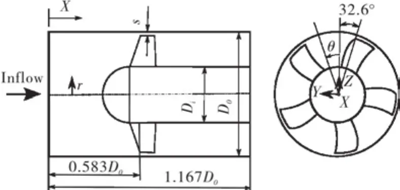
Fig.2 Schematic of the 5-bladed axial fan

Fig.3 Axial fan geometry and detailed view of the mesh around the blade

The Reynolds number isRe==9.36×105based on the densityρ,the viscosityηof the incoming flow,and the rotational speed ofn=3 000rpm.The operating point is defined by a volume flow rate ofV=0.65m/s.Furthermore,the inner diameter isDi=0.135m and the outerDo=0.3m.The computations have been performed for two gap sizes withs/Do=0.01 ands/Do=0.005 using 8 192 Processors on the CRAY System HERMIT at the High Performance Computing Center in Stuttgart(HLRS).A detailed view of the grid resolution for both tip-gap configurations is shown in Fig.4.

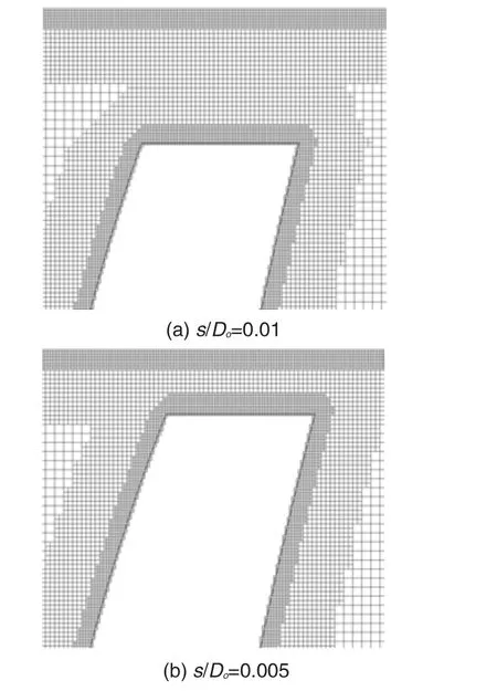
Fig.4 Computational mesh of the grid near the tip-gap region fors/Do=0.01 ands/Do=0.005

2.4 Boundary Conditions

2.4.1 Inlet,outlet,and walls

At the inlet,the mass flow is prescribed and the streamwise pressure gradient is set to zero.At the outlet,a fixed static pressure is prescribed and all other variables are extrapolated from the internal field.Sponge layers are applied to damp numerical reflections caused by the inlet and outlet boundaries.At all walls,a no-slip condition with zero pressure and density gradients in the wall normal direction is imposed.

2.4.2 Periodic Boundary Condition for Cartesian Meshes

Since Cartesian grids do not allow a simple rotationally periodic condition except for integer multiples of 90°,a boundary condition for arbitrary angles was formulated and implemented for refined hierarchical Cartesian meshes.Fig.5 shows a simple two-dimensional 72°rotational periodic domain,which is decomposed into four subdomains for parallel computation.The periodic boundary is marked by red lines.For the application of the boundary condition,an overlapping region with at least two cell layers is used to maintain an accuracy of second-order for all spatial gradients.Cells with a center located outside of the red lines are marked as periodic cells and all primitive variables of these cells are updated after each Runge-Kutta step.

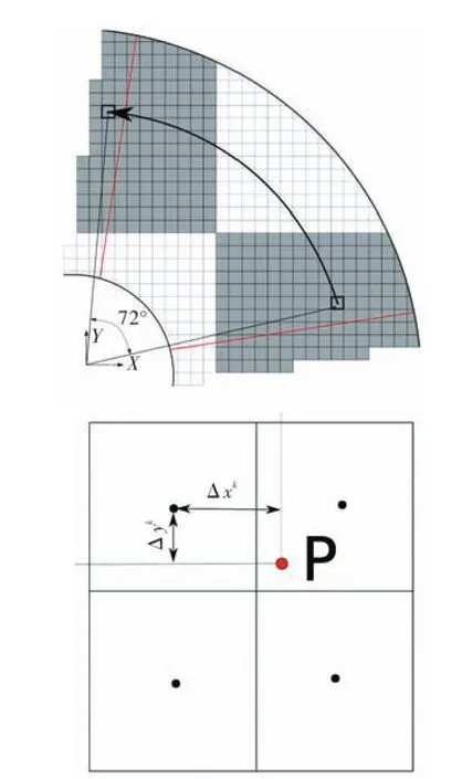
Fig.5 Schematic of the periodic boundary condition

In a first step,the coordinate of each periodic cell is rotated by 72°and sent to all available processors working on the simulation.The rotated coordinate is marked byPin Fig.5.Each processor checks whetherPis inside its subdomain.If so,an internal cell surrounding the coordinatePis determined.For this purpose,a kd-tree search algorithm is used which allows to find these cells in logarithmic time.Once corresponding cells are found for all periodic cells,a connectivity matrix is generated on each processor such that the cell data can be determined subsequently without searching and exchanging between the corresponding subdomains.Since the cells centers of the rotated periodic cell and the corresponding internal cell typically do not match,each primitive variableξis reconstructed from its neighbor cells using a non-linear least-squares method.This involves the solution of a linear equation system

whereNdenotes the number and△xkand △ykand denote the distance between thek-th reconstruction cell and the coordinateP.Two layers of cell neighbors are used for the reconstruction.After solving the linear system,the value of the primitive variable at coordinatePis given by ζP=α0.This procedure can be directly extended to three space dimensions.After the reconstruction,the primitive variables are exchanged with the other domains.

The periodic boundary condition has been tested for a laminar pipe flow at a Reynolds numberRe==100,whereUbis the bulk velocity.The pipe length is chosen asL/D=10.The computation has been performed for a 72°pipe segment and for a full domain with 360°.The axial velocity profiles at different circumferential positions in Fig.6 show a good agreement between both computations and the analytical solution.

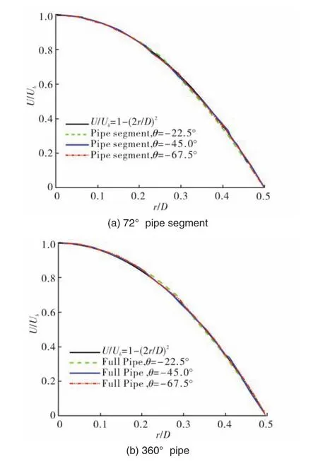
Fig.6 Velocity profiles of pipe flow at different circumferential positions

3 Results

3.1 Grid Convergence Study

For the grid convergence study computations are performed for a fixed operating point defined by a constant flow coefficientϕ==0.165.For this case the Reynolds number based on the relative velocity of the outer casing wall isRe=πD20n/v=9.36×105.Two different meshes are used for the computations,i.e,case d with 2.5×108cells and case e with 1×109cells.Computational resources for both cases are summarized in Table 1.The simulations were conducted on 7 992 computing cores for mesh case d and 31 992 computing cores for mesh case e.The time step for both cases isΔt=1.936×10-5and the number of time steps corresponding to four full rotations of the rotor is 0.64×106resulting in a wall clock time of approx.250h for each computation.After two full rotations 2 000 samples of instantaneous data were collected for statistical analysis.

Tab.1 Computational details of the fan simulation,including the disk space for 2 000 samples used to determine the turbulence statistics.

Fig.3 illustrates an example of the computational grid for the 72°fan section and highlights the resolution and refinement of the grid in wall regions.Fig.7 depicts the experimental operating line of the fan showing the pressure coefficientas a function of the flow coefficientΦ,whereΔp=pstat,out-p0,in,i.e.,the difference of the static pressure at the outletpstat,outand the stagnation pressureattheinletp0,inofthefan.Asshown,bothnumerical results agree well with the experiment.， whereΔp=pstat,out-p0,in,i.e.,the difference ofthe static pressure atthe outletpstat,outand the stagnation pressure at the inletp0,inof the fan,versus the flow coefficientΦ=;experimental data from[16].

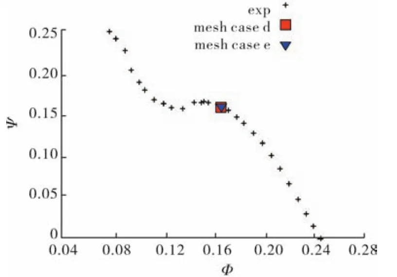
Fig.7 Operating map for a constant tip-gap size of s/D0=0.01 showing the pressure coefficient

To give an impression of the overall flow field,Fig.8(a)depicts the instantaneous contours of the Q-criterion[17]visualizing the vortical structures.Several physical phenomena are evident,e.g.,a development of a passage vortex on the blade root initiating a transition of the incoming boundary layer,a turbulent wake behind the trailing edge of the blade,a transition region on the blades suction side and a jet-like tip-gap vortex due to the leakage flow through the tip-gap generating a turbulent wake region.The flow field inside the tip-gap is caused by the pressure difference between the pressure and the suction side as illustrated by Fig.8(b) which shows the instantaneous contours of the pressure coefficientin the gap region,wherepinis the mean inlet pressure.Low pressure regions are observed inside the tip-gap due to separations on the surface of the blade tip and upstream of the blade due to the tip-gap vortex.

Fig.8 Instantaneous contours of(a)the Q-criterion showing the vortical structures around the blade and(b)the pressure coefficient showing low pressure regions caused by the tip-gap vortex and the separation vortices inside the tip-gap for mesh case e

To analyze the impact of the grid resolution Fig.9 shows the time-averaged relative Mach number contours at a constant axial locationx/D0=0.617 for mesh case d and e.A marginal impact of the grid resolutions on the Mach number contours in Fig.9 is observed.For both mesh cases,the Mach number increases in the radial direction and drops in the wake generated by the tip-gap vortex.A maximum Mach number is observed near the tip-gap region.

Fig.9 Mean relative Mach number contours at a constant axial locationx/D0=0.617

To further quantify the impact of the mesh,Fig.10 and Fig.11 show axial distributions of the pressure coefficient and the turbulent kinetic anergy at 80%span and two circumferential locations,i.e., Θ =-45°and Θ =-35°.Upstream of the blade,the pressure coefficients in Fig.10 shows a smooth drop due to the suction region.Larger values are observed on the pressure side of the blade,as already observed in Fig.8(b).The impact of the mesh on the pressure coefficient negligibly small and the curves almost perfectly match for both locations.The turbulent kinetic energy distribution in Fig.11 shows high values on pressure side of the blade due to the turbulent wake generated by tip-gap vortex of the neighboring blade.Only a small impact of the grid resolution at both location its observed.

Fig.10(a)Axial distribution of the pressure coefficient atΘ=-45°and 80%span;(b)Axial distribution of the pressure coefficient atΘ=-35°and 80%span.Mesh case d(-),mesh case e(-·-).

Fig.11 (a)Axial distribution of the turbulent kinetic energy atΘ=-45°and 80%span;(b)Axial distribution of the turbulent kinetic energy atΘ=-35°and 80%span.Mesh case d(-),mesh case e(-·-).

3.2 Volume Flow Rate Variation

In this section the impact of the flow coefficient on the flow field near the tip-gap region is demonstrated for mesh case d.Fig.12 and 13 show the time-averaged Mach number contours including streamlines of the projected velocity vector and the turbulent kinetic energy contours in several radial planes fromϕ=-30°toθ=-60°,forϕ=0.165 andϕ=0.195.Forϕ=0.195,the tip-gap vortex passes by the leading edge of the neighboring blade without any interaction.

Fig.12 Time-averaged contours of Mach number contours and streamlines of projected velocity vector in different radial planes from θ=-30°toθ=-60°,forϕ=0.165(left)andϕ=0.195(right).

Fig.13 Turbulent kinetic energy contours in several radial planes from θ=-30°toθ=-60°,forϕ=0.165(left)andϕ=0.195(right).

Asmallcounter-rotatingseparationvortexappearsnear the leading edge,which,however,has a very low turbulent kinetic energy such that a marginal effect compared to the wake,which impinges upon the blade for the lower volume flow rate,is observed.Forϕ=0.165,the tip-gap vortex,which has a larger diameter and is more turbulent,spreads in the axial direction and breaks up in two vortices,where the left vortex is fed by the right vortex and grows.Subsequently,the turbulent left vortex interacts with the leading edge of the blade,which causes strong fluctuations near the gap region extending further upstream compared toϕ=0.195.This results in a larger tip-gap vortex with a higher turbulent kinetic energy,which is created due to the back flow caused by the adverse pressure gradient,supporting the turbulent transition on the suction side.For both volume flow rates,a counter rotating separation vortex is observed next to the tip-gap vortex,which disappears earlier forϕ=0.165.

In addition,Fig.14 depicts the radial distribution of the Mach number and the turbulent kinetic energy inside the tip-gap atx/D0=0.617 andθ=-45°.The results forϕ=0.165 show a lower Mach number and a higher turbulent kinetic energy inside the tip-gap.

Fig.14 Radial distribution of Mach number(a)and turbulent kinetic energy(b)inside the tip-gap atx/D0=0.617 andθ=-45°,forϕ=0.165(-)andϕ=0.195(--).

3.3 Comparison of LES and RANS Results

We start by presenting LES results of the instantaneous and time-averaged flow field fors/D0=0.01.Then,the time-averaged flow field quantities are compared to RANS results[18],which were determined by the flow solver THETA developed at the German Aerospace Center DLR[19].The THETA-code is a Finite-Volume method for solving the RANS equations for incompressible flow.The method uses unstructured grids with tetrahedral or prism shaped cells and a colocated variable arrangement.The interpolation scheme of Rhie and Chow[20]is used to avoid a decoupling of the solution variables.The convective fluxesare discretized using the centraldifferencing scheme(CDS)or using different upwind schemes,i.e.linear upwind scheme(LUDS)andquadraticupwind scheme(QUDS).The projection method is used for the velocity pressure coupling.The BiCGStab method or the FGMRES method with a multi-grid preconditioner is used to solve the linear systems of the momentum,pressure and turbulence equations.To close the RANS equations,the SST k-ω model of Menter et al.[21]was used.Finally,the influence of the tip-gap size on the vortical structures based on LES results is discussed by reducing the gap size tos/D0=0.005.

For all computations,the Navier-Stokes equations are solved in a rotating frame of reference,with a rotating outer wall and a fixed blade position.Therefore,all the velocities and Mach numbers in the following are based on the rotating reference frame.The simulations have been performed for a non-dimensional time corresponding to two full rotations of the rotor using 8 192 computing cores.After a fully developed flow field was obtained and 320 samples were recorded during another two full rotations for the statistical analysis of the flow data.Fig.15 depicts the operating map of the axial fan showing the pressure coefficient versus the flow coefficient for two tip-gap sizes.Due to the higher losses the operating line for the larger tip-gap is shifted to lower values of the pressure coefficients.The LES results,which are denoted by green marks are in good agreement with the experiment.The RANS result,which was obtained for the larger tip-gap and is denoted by a red mark slightly underpredicts the pressure gain.

In Fig.16 the contours of the instantaneous relative Mach number distribution in a plane at a constant axial positionx/D0=0.63 fors/D0=0.01 are shown.The 72°section was duplicated to show that the solution is fully periodic and smooth across the periodic boundary,which is denoted by a red line.A high Mach number region with a turbulent wake can be observed near the tip-gap.

Fig.15 Operating map for two tip-gap sizess/D0=0.01 and s/Do=0.005, showing the pressure coefficient,whereΔp=pstat,out-p0,in,i.e.,the difference ofthe static pressure atthe outlet pstat,out and the stagnation pressure at the inletp0,inof the fan,versus the flow coefficient

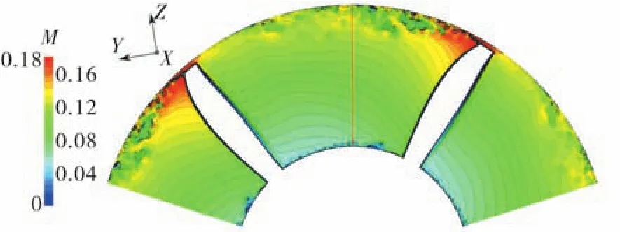
Fig.16 Contours of the instantaneous relative Mach number distribution across the periodic boundary atx/D0=0.63 fors/D0=0.01.

In Fig.17 instantaneous contours of the Q-Criterion[17]colored by the velocity magnitude fors/D0=0.01 are shown.A main tip-leakage vortex,which expands downstream,and several tip-separation vortices,which interact with the tip-leakage vortex,are observed.Furthermore,a transition region occurs at the hub.To have a closer look at the vortex structures,Fig.18 illustrates time-averaged values of the axial velocity u with streamlinesoftheprojected velocity vector,the turbulent kinetic energy k,and the vorticity magnitude|in three planes along the chord,at the inclination anglesθ1=-45°,θ2=-40°,andθ3=-35°fors/D0=0.01.

Fig.17 Instantaneous contours of the Q-criterion in the tip-gap region colored by the velocity magnitude fors/D0=0.01

All three planes cross the centerline and are parallel to the x-axis.Additionally,the time-averaged contours of the Q-criterion are illustrated by red lines in Fig.18,to visualize the location of the vortices.In the first plane atθ3=-45°,the formation of three types of vortices similar to the studies of You et al.[6]and Boudet et al.[8]is observed.The largest vortex is the tip-leakage vortex on the suction side.The turbulent kinetic energy k increases as the vortex grows along the chord.The change of the vorticity magnitudealong the chord,however,is negligible.Additionally,a slower growing counter-rotating passage vortex due to a separation at the casing wall is evident.The main source of the turbulent kinetic energy k is the small separation vortices on the surface of the blade tip.The quantities k and |peak in this region.

Fig.18 Contours of the time-averaged axial velocity u with streamlines of the projected velocity vector(top),turbulentkinetic energy k(center),and vorticity magnitude(bottom)atθ1=-45°(left),θ2=-40°(center),andθ3=-35°(right)fors/D0=0.01.

Results of the time-averaged flow field compared to RANS results fors/D0=0.01 are presented in Fig.19.In Figs.19(a)and(b)the axial distribution of the pressure coefficient based on the inlet pressureand the axial Mach number distribution at midspan and a constantcircumferentialpositiondefinedbyθ=-45°according to Fig.2 are shown.Additionally,the radial relative Mach number distributions at three axial positions andθ=-45°are depicted in Figs.19(c)～(e).In Fig.19(e)the wake near the outer wall caused by the tip-leakage vortex is illustrated.Fig.19(f)shows a radial distribution of the turbulent kinetic energy at a fixed position inside the wake region.Two peaks are evident in the distribution,one at the hub wall,which indicates a turbulent boundary layer,and another peak at the outer wall,which is much higher and is caused by the tip-leakage vortex.The main differences between RANS and LES are located in the wake region.In all other regions,LES and RANS are in good agreement.A larger difference is observed in the distribution of the turbulent kinetic energy k.At the hub,the difference of k between LES and RANS is small,but near the casing wall,where the flow is highly unsteady due to the tip-leakage vortex,k is approx.3 times higher in the LES.

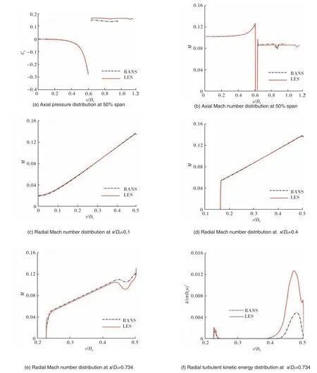
Fig.19 Comparison between RANS and LES results of the time-averaged flow field fors/D0=0.01 atθ=-45°

To investigate the influence of the tip-gap size on the vortical structures another LES computation with a smaller tip-gap ofs/D0=0.005 was performed.Fig.20 shows the contours of the time-averaged Q-criterion colored by the vorticity in the azimuthal directionωθfors/D0=0.01 ands/D0=0.005.

The colors red and blue denote different rotational directions,where red is used for positiveωθand blue for negativeωθ.In both cases,a main tip-gap vortex and several separation vortices in the tip-gap can be observed.However,for the larger tip-gap in Fig.20(a)the tip-gap,vortex is almost straight,whereas for the smaller tip-gap the tip-gap vortex is curved and follows the contour of the airfoil.Furthermore,a counter-rotating separation vortex upstream of the tip-gap vortex is present,which is much shorter and occurs further off the leading edge for thes/D0=0.01.Due to the smaller tip-gap more separation vortices followed by small counter-rotating vortices occur inside the tipgapfors/D0=0.005,whichinteractwiththetip-gapvortex.As shown in Fig.21,that illustrates the time-averaged relative Mach number contours and streamlines of the projected velocity vector in several radial planes fromθ=-30°toθ=-70°fors/D0=0.01 ands/D0=0.005,the initial angle of attack of the tip-gap vortex relatively to the blade is larger for the smaller tip-gap,but due to its strong curvature it passes the neighboring blade further downstream.Although there are more separation vortices interacting with each other for the smaller tip-gap,the diameter of the tip-gap vortex is much smaller compared to the tip-gap vortex fors/D0=0.01.

Fig.20 Time-averaged contours of the Q-criterion colored by the vorticity in the azimuthal direction ωθnear the tip-gap region fors/D0=0.01(left)ands/D0=0.005(right).The color red denotes positive ωθand blue negative ωθto indicate the rotational direction of the vortices.

Fig.21 Time-averaged contours of the relative Mach number and streamlines of projected velocity vector in differentradialplanesfrom θ=-30°to θ=-70°,fors/D0=0.01(a)ands/D0=0.005(b).

Fig.22 Turbulent kinetic energy contours in several radial planes from θ=-30°toθ=-70°,fors/D0=0.01(a)ands/D0=0.005(b).

Additionally,decreasing the tip-gap results in fewer losses as illustrated in Fig.22 by the turbulent kinetic energy in different radial planes fromθ=-30°toθ=-70°fors/D0=0.01 ands/D0=0.005.The turbulent kinetic energy caused by several small separation vortices and the smaller tip-gap vortex is lower than for the larger tip-gap.

Fig.23 depicts the axial distributions of the relative Mach number and turbulent kinetic energy at three radial positions(20%,50%,and 80%span)andθ=-45°.Solid lines are used fors/D0=0.005 and dashed lines fors/D0=0.01.Upstream of the blade forx/D0＜0.6,no influence of the tip-gap size on the Mach number can be observed at 20%and 50%span.At 80%span,the Mach number for the smaller tip-gap is slightly higher towards the suction side of the blade for the smaller tip-gap.For both cases the turbulent kinetic energy is zero upstream of the blade.Forx/D0＞0.6,the Mach number distributions at 20%and 50%span are similar for both tip-gaps.However,fors/D0=0.005 the Mach number distributions are slightly shifted towards lower values.The turbulent kinetic energy distributions are almost alike at 20%and 50%span.As expected,the largest influence on the Mach number and turbulent kinetic energy can be observed at 80%span due to the strong differences of the turbulent wakes caused by the different vortical structures near the tip-gap.Fig.24 shows the radial distribution of the relative Mach number and turbulent kinetic energy inside the tip-gap atx/D0=0.617 andθ=-45°.

Fig.23 Axial distribution of the relative Mach number(left)andturbulentkineticenergy(right)atθ=-45°and three radial positions(20%,50%,and 80%span)fors/D0=0.005(solid)ands/D0=0.01(dashed).

Fig.24 Radial distribution of the relative Mach number(left)and turbulent kinetic energy(right)inside the tip-gap atx/D0=0.617 and θ=-45°,fors/D0=0.005(solid)ands/D0=0.01(dashed).

The maximum Mach number almost matches for both tip-gap sizes.Near the tip of the blade,forr/s＜0.5 however,the Mach number is lower fors/D0=0.005 and strongly decreases towards the wall.Furthermore,the peak of the turbulent kinetic energy is located further away from the tip surface and is lower by a factor of two.

4 Computational Details

In the present paper,the Zonal Flow Solver(ZFS)has been used,which is an in-house code of the Institute of Aerodynamics.Its mesh structure is based on an unstructured hierarchical octree data structure.Such a data structure requires more computing time per cell compared to flow solvers on structured meshes due to the indirect and more random memory access.The unstructured mesh system,however,allows to mesh complex geometries,such as highly skewed blades,or full turbine stages without introducing manual mesh generation effort.For the axial fan computational meshes were generated fully automatically with more than 1×109cells.In addition,the domain decompositioning,which is based on a space filling curve,generates compact subdomains for any number of computing cores.A strong scaling test has been performed on the HLRS Cray XC40 Hornet for the axial fan configuration.

The simulation were carried out on Intel Xeon CPUs E5-2 680v3,where each node with a dual CPU has 24 physical cores operating at 2.50 GHz.In the present test,thenumbergridpointsareapprox.1.0×109cells.Thescaling test has been performed from 228 to 3 828 nodes,i.e.,a total number of 5 472 to 91 872 CPU cores has been used.The scaling results are shown in Fig.25.

Fig.25 Strong scaling speedup test

Tab.2.Strong scaling measurements

The shown speed-up behavior is not perfect for higher core numbers.In that case the cells involved in the periodic boundary condition generate a higher workload on a few subdomains,which produces a load imbalance increasing with the number of CPU cores.A domain decompositioning taking into account the additional work for these cells or a dynamic load balancing based on the actual computing time per subdomain would improve the parallel efficiency.Such a load balancing procedure is presently being implemented in ZFS.

5 Conclusion

LES results of the turbulent flow around a rotating axial fan were presented and compared to a RANS solution.The LES solution method is based on hierarchical Cartesian meshes.The simulations were performed for a 72°segment including only one blade of the fan.This segment solution required an implementation of a parallelized rotational periodic boundary condition which has been introduced andvalidatedforasimplelaminarpipeflowatalowReynolds number.A smooth and rotational periodic solution across the periodic boundary confirmed its applicability to axial fan flow.The major vortices in the tip-gap region,the tip-leakage vortex,the counter-rotating passage vortex,and the separation vortices could be resolved by the LES.The comparison of the LES results of the mean flow field to the RANS solution showed differences primarily in the wake region of the fan,especially for the turbulent kinetic energy k.In addition,a computation with a smaller tip-gap size has been performed.The largest differences in the flow field could be observed at high spanwise locations in the wake region,where the flow field is dominated by the vortical structures caused by the tip-gap.Reducing the tip-gap results in a smaller tip-gap vortex which follows the contour of the blade more closely and the development of more separationvorticesfollowedbycounter-rotatingvortices.The turbulent kinetic energy and therefore the losses near and insidethetip-gaparereducedforthesmallertip-gap.

[1]Carolus,T.,Schneider,M.,and Reese,H.,Axial flow fan broadband noise and prediction,"Journal of Sound and Vibration,Vol.300,No.1-2,2007,pp.50 70.

[2] Reese, H., Anwendung von instationaren numerischen Simulationsmethoden zur Berechnung aeroakustischer Schallquellen bei Axialventilatoren,Ph.D.thesis,University of Siegen,2007.

[3]Reese,H.and Carolus,T.,Axial Fan Noise:Towards Sound Prediction Based on Numerical Unsteady Flow Data-a Case Study,"Euronoise Paris,2008,pp.4069{4074.

[4]You,D.,Mittal,R.,Wang,M.,and Moin,P.,Large-eddy simulation of a rotor tip-clearance flow,"AIAA Paper 2002-0981,2002.

[5]You,D.,Mittal,R.,Wang,M.,and Moin,P.,Computational methodology for large-eddy simulation of tip-clearance flows,"AIAA Journal,Vol.42,No.2,2004,pp.271{279.

[6]You,D.,Wang,M.,Mittal,R.,and Moin,P.,Study of rotor tipclearance ow using large eddy simulation,"AIAA Paper 2003-0838,2003.

[7]You,D.,Wang,M.,Moin,P.,and Mittal,R.,E ects of tip-gap size on the tip-leakage flow in a turbomachinery cascade,"Physics of Fluids,Vol.18,No.10,2006,pp.105102.

[8]Boudet,J.,Caro,J.,and Jacob,M.,Large-eddy simulation of a single airfoil tip-clearance flow,"16th AIAA/CEAS Aeroacoustics Conference,AIAA Paper 2010-3978,Stockholm,2010.

[9]Cahuzac,A.,Boudet,J.,and Jacob,M.,Large-Eddy Simulation of a rotortip-clearance flow,"17th AIAA/CEAS Aeroacoustics Conference,AIAA Paper 2011-2947,2011.

[10]Lintermann,A.,Schlimpert,S.,Grimmen,J.H.,Gunther,C.,Meinke,M.,and Schroder,W.,Massively Parallel Grid Generation on HPC Systems,"Computer Methods in Applied Mechanics and Engineering,Vol.277,2014,pp.131{153.

[11]Hartmann,D.,Meinke,M.,and Schroder,W.,A strictly conservative Cartesian cut-cell method for compressible viscous flows on adaptive grids,"Computer Methods in Applied Mechanics and Engineering,Vol.200,No.9-12,2011,pp.1038{1052.

[12]Meinke,M.,Schroder,W.,Krause,E.,and Rister,T.,A comparison of second-and sixth-order methods for large-eddy simulation,"Computers and Fluids,Vol.31,No.4-7,2002,pp.695 718.

[13]Jameson,A.and Mavriplis,D.,Finite volume solution of the twodimensional Euler equations on a regular triangular mesh,"AIAA Journal,Vol.24,No.4,1986,pp.616{618.

[14]Schneiders,L.,Hartmann,D.,Meinke,M.,and Schroder,W.,An accurate moving boundary formulation in cut-cell methods,"Journal of Computational Physics,Vol.235,2013,pp.786 809.

[15]Sturm,M.and Carolus,T.,Tonal Fan Noise of an Isolated Axial Fan Rotor due to Inhomogeneous Coherent Structures at the Intake,"Noise Control Engineering Journal,Vol.60,No.6,2012,pp.699 706.

[16]Zhu,T.and Carolus,T.,Experimental and Numerical Investigation of the Tip Clearance Noise of an Axial Fan,"Paper No.GT2013-94100,2013.

[17]Jeong,J.and Hussain,F.,On the Identi cation of a Vortex,"Journal of Fluid Mechanics,Vol.285,1995,pp.69 94.

[18]Pogorelov,A.,Meinke,M.,Schrder,W.,and Kessler,R.,Cut-Cell Method Based Large-Eddy Simulation of a Tip-Leakage Vortex of an Axial Fan,"AIAA Paper 2015-1979,2015.

[19]Knopp,T.,Zhang,X.,R.,K.,and G.,L.,Enhancement of an industrial nite-volume code for large-eddytype simulation of incompressible high Reynolds number flow using near-wall modelling," ComputerMethodsin Applied Mechanicsand Engineering,Vol.199,2010,pp.890 902.

[20]Rhie,C.M.and Chow,W.L.,Numerical study of the turbulent flow past an airfoil with trailing edge separation,"AIAA Journal,Vol.21,1983,pp.1525 1532.

[21]Menter,F.R.,Kuntz,M.,and Langtry,R.,Ten Years of Industrial Experience with the SST Turbulence Model,"Turbulence,Heat and Mass Transfer 4,edited by K.Hanjalic,Y.Nagano,and M.Tummers,Begell House,Inc.,2003,pp.625 632.