A Dimensional Splitting Method for 3D Elastic Shell with Mixed Tensor Analysis on a 2D Manifold Embedded into a Higher Dimensional Riemannian Space

Kaitai Li and Xiaoqin Shen

1 School of Mathematical Sciences and Statistics,Xi’an Jiaotong University,Xi’an,710049,P.R.China.

2 School of Sciences,Xi’an University of Technology,Xi’an,710048,P.R.China.

Abstract.In this paper,a mixed tensor analysis for a two-dimensional(2D)manifold embedded into a three-dimensional(3D)Riemannian space is conducted and its applications to construct a dimensional splitting method for linear and nonlinear 3D elastic shells are provided. We establish a semi-geodesic coordinate system based on this 2D manifold,providing the relations between metrics tensors,Christoffel symbols,covariant derivatives and differential operators on the 2D manifold and 3D space,and establish the Gateaux derivatives of metric tensor,curvature tensor and normal vector and so on,with respect to the surface →Θ along any direction→η when the deformation of the surface occurs.Under the assumption that the solution of 3D elastic equations can be expressed in a Taylor expansion with respect to transverse variable,the boundary value problems satisfied by the coefficients of the Taylor expansion are given.

Key words:Dimensional splitting method,linear elastic shell,mixed tensor analysis,nonlinear elastic shell.

1 Introduction

A shell is a three-dimensional(3D)elastic body that is geometrically characterized by its middle surface and its small thickness.The middle surface ℑ is a compact surface in ℜ3that is not a plane(otherwise the shell is a plate),and it may or may not have a boundary.For instance,the middle surface of a sail has a boundary,whereas that of a basketball has no boundary.

At each point s ∈ℑ,let n(s)denote a unit vector normal to ℑ. Then the reference configuration of the shell,(that is,the subset of ℜ3that occupies before forces are applied to it),is a set of the formwhere the function e:ℑ→ℜ is sufficiently smooth and satisfiesfor all s∈ℑ.Additionally,ε＞0 is thought of as being‘small’compared with the‘characteristic’length of ℑ(its diameter,for instance).If e(s)=ε,∀s∈ℑ,the shell is said to have a constant thickness of 2ε.If e is not a constant function,the shell is said to have a variable thickness.

The theory of elastic plates and shells is one of the most important theories of elasticity.Thin shells and plates are widely used in civil engineering projects as well as engineering projects.Examples include aircraft,cars,missiles,orbital launch systems,rockets,and trains.

Considerable work on the subject was conducted by the Russian scholars A.I.Lurje(1937),V.Z.Vlasov(1944)and V.V.Novozhilov(1951)after the pioneer idea of Love.However,now it appears necessary to improve the mathematical understanding of the classical plate and shell models pioneered by these scholars.The reason for this is that the precision required in aircraft and spacecraft projects has intensified with the advent of powerful electronic computers.The goal therein is,on the one hand,to develop better finite approximations on elements and,on the other hand,to refine theoretical models when necessary.

A.L.Gol’denveizer(1953)first put forward the ideas of conducting an asymptotic analysis based on the thickness of a shell or plate.New formulations for shells and plates were obtained by relaxing the constitutive relations and reinforcing the equilibrium that must be satisfied.Even in presenting a much more detailed analysis than that offered by his predecessors,no mathematical justification was given by Gol’denveizer.As such,a large number of difficulties were still to be overcome.At the same time,the weak formulations of J.L.Lions and mixed formulations of Hellinger-Reissner and Hu-Washizu(1968)appeared to provide alleviation.Of particular significance was the work of J.L.Lions(1973)on singular perturbation,which provided the tools and explanation for what happens when the asymptotic method is applied to plates,shells,and beams.The mathematical foundation of elasticity can be found in[4,6].The asymptotic method was revisited in a functional framework proposed by Li,Zhang and Huang[1],P.G.Ciarlet[3,4]and M.Bernadou[5].Their work made convergence and error analysis possible therein for the first time.

The 3D models are derived directly from the principles of equilibrium in classical mechanics,and are viewed as singular perturbation problems dependent upon the small parameter ε(the half-thickness of the shell).2D models are obtained by making some additional hypotheses that are not justified by physical law.Our aim here is to justify mathematically the assumptions that formulate the basis of a 2D model of elasticity,and whose solution approaches 3D displacement better than the solution of classical models.

This paper is organized as follows:in Section 2,we present a mixed tensor analysis on 2D manifolds embedded into 3D Euclidian space;in Section 3,we provide the exchange of tensors and curvature after the deformation of curvatures;in Section 4,we give differential operators in 3D Riemannian space under semi geodesic coordinate system;in Section 5,asymptotic forms of 3D linear and nonlinear elastic operators with respect to transverse variable ξ are derived;in Section 6,a specific shell as an example,is provided.

2 Mixed tensor analysis on a 2D manifold embedded into a 3D Riemannian space

Tensor analysis in Riemannian space can be found in[2]. Here it presents for mixed tensor analysis on a 2D manifold embedded into a 3D Riemannian space,in which we provide basic theorem and formula and gives proof in details.

Let us consider elastic shells,which is assumed to be a St Venant-Kirchhoff material and homogeneous and isotropic.Hence this material is characterized by its two Lam´e constants λ＞0 andµ＞0 which are thus independent of its thickness.

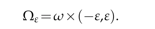
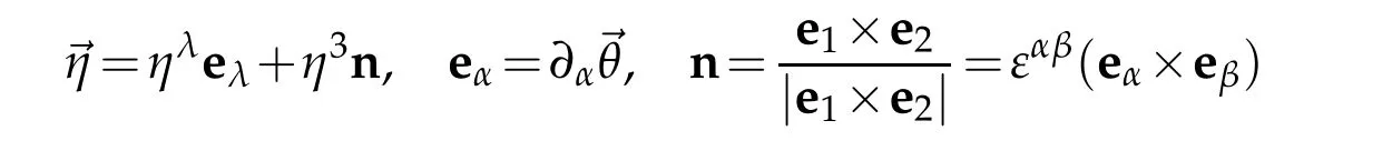
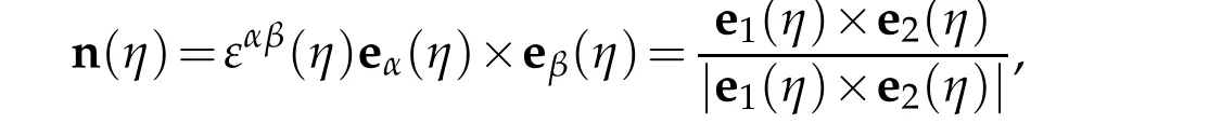
An elastic shell whose reference configuration(3D-Euclidean space)consists of all points within a distance ≤ε from a given surface ℑ ⊂E3and ε ＞0 which is thought of being small.The 2D manifold ℑ⊂E3is called the middle surface of the shell,and the parameter ε is called the semi-thickness of the shell.The surface ℑ can be defined as the image →θ of the closure of a domain ω ⊂R2,where →θ:¯ω →E3is a smooth injective mapping.Let→n denote an unit normal vector along ℑ and let

The pair(x1,x2)is usually called Gaussian coordinate on ℑ,and(x1,x2,ξ)is called semigeodesic coordinate system(S-Coordinate System)(if E3is a Riemmannian space andℑ is a 2D manifold). The boundary of shellconsists as follows: ·top surface Γt=ℑ×{+ε},

·bottom surface Γb=ℑ×{-ε},

·lateral surface Γl=Γ0∩Γ1:Γ0=γ0×{-ε,+ε},Γ1=γ1×{-ε,+ε},where γ=γ0∪γ1is the boundary of ω:γ=∂ω.

In what follows,Latin indices and exponent:(i,j,k,···)take their values in the set{1,2,3}whereas Greek indices and exponents(α,β,γ,···,)take their values in the set{1,2}. In addition,Einstein’s summation convention with respect to repeated indices and exponent is used.

It is well known that the covariant and contravariant component of the metric tensors on the surface ℑ are given by

Furthermore,it is well known that the contravariant components of bαβ,cαβare given by

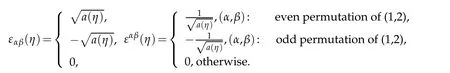
which will play important role in the followings.In the same season we have to introduce permutation tensors in ℜ3and on ℑ which are given by

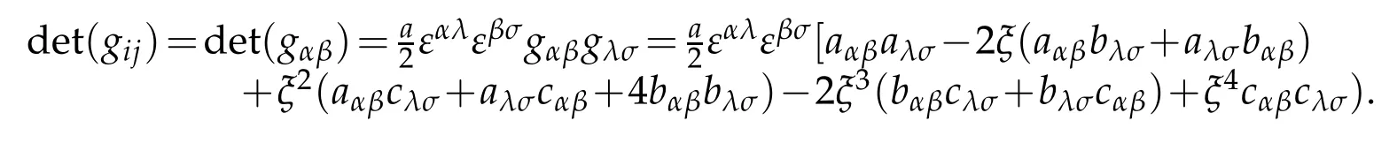
where g=det(gij)and gijis metric tensor of ℜ3.

Similarly

Let H and K denote mean curvature and Gaussian curvature respectively:

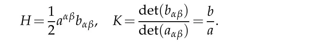
Then the determinant of third fundamental tensor cαβis

Using permutation tensors in ℜ3and on ℑ the following relationships are held

and

The following lemma present fundamental formula concerning many basic tensors of order two on the surface.

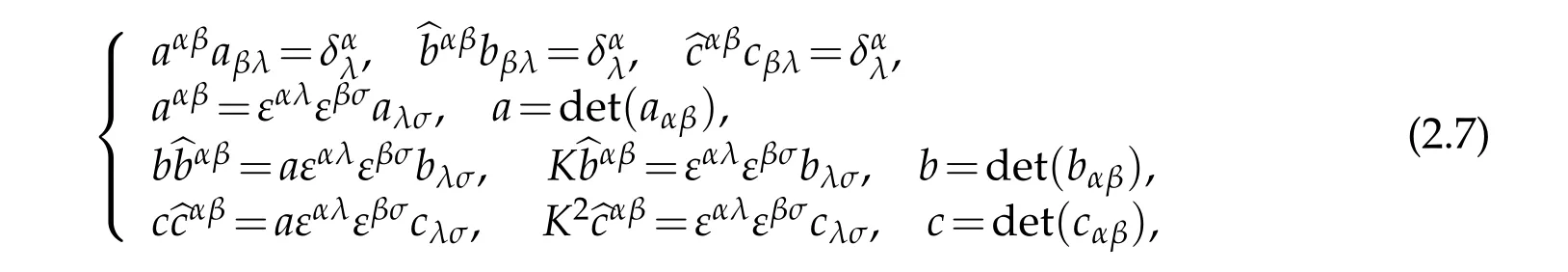
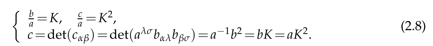
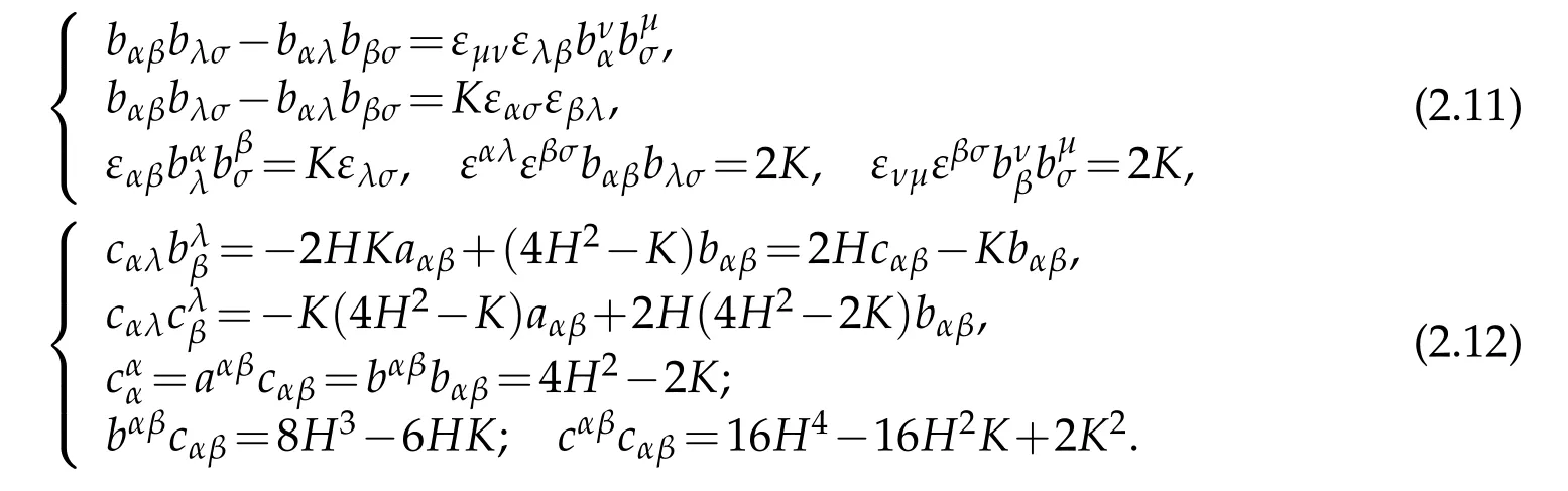
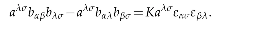
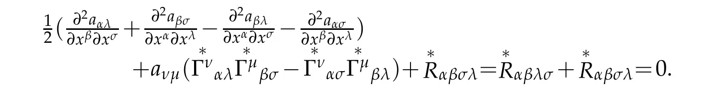
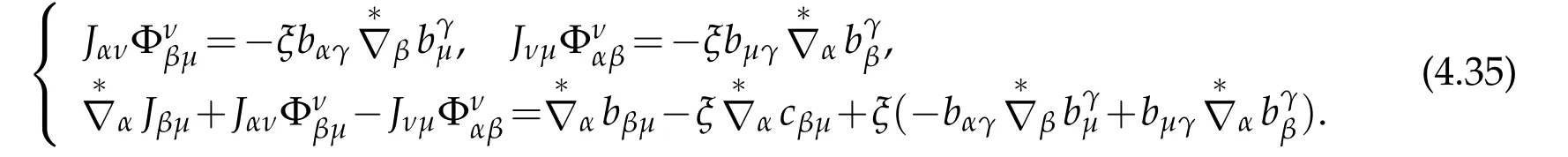
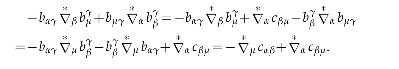
Lemma 2.1.The third fundamental tensor is not independent of the first and second fundamental tensors aαβ,bαβ.There are following relationships

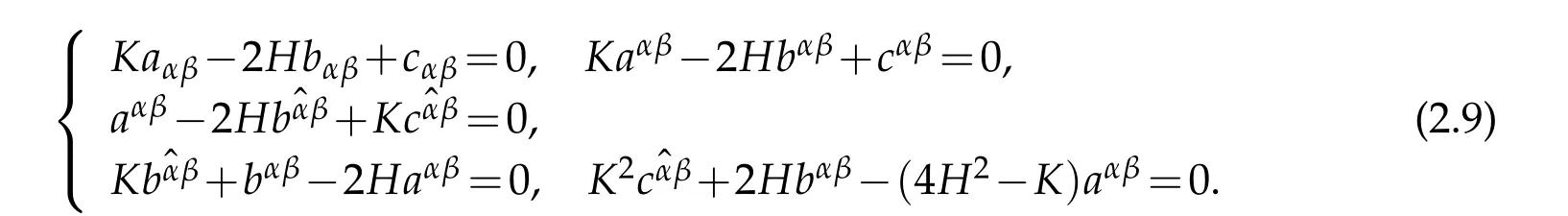
Besides,there are relationships between matrices bαβ,cαβand its inverse matricesas follows

Furthermore,

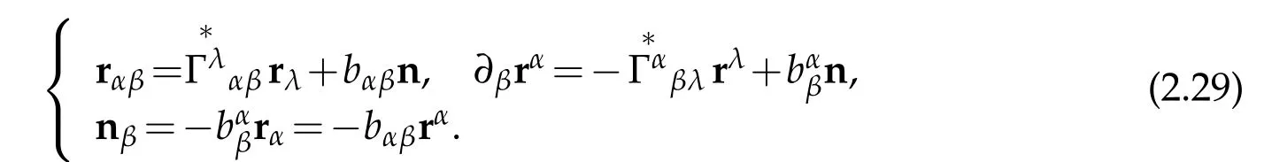
Proof.First,we prove(2.11).For the simplicity,let r=→θ and n denote the unite normal vector to surface ℑ.(2.3)shows bαβ=-nαrβ,therefore

In terms of formula in vector analysis

it yields that

On the other hand,applying Weingarten formula

and permutation tensor

we can obtain

This is the first part of(2.11).

Next we prove last two formula in(2.11).Remember that

Therefore,

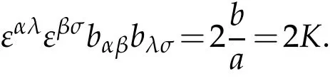
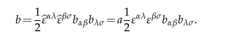
This is the forth part of(2.11).Using εαλaανaλµ=ενµwe derive

This is the fifth part of(2.11).

Applying εβλto contraction of indices of tensor for both sides of above equality

This is the third part of(2.11).

Next,we prove second of(2.11).To do that,combing the first and third part of(2.11),we have

From this it yields the second part of(2.11).

Next we prove(2.9).To do that by contraction of tensor indices for the second part of(2.11)with aλσwe have

Because of

we can obtain the first part of(2.9).

Using the trick of tensor indices left leads to the second part of(2.9).

In order to prove the third part of(2.9),multiplying both sides of tensor index of the first part of(2.9)by εαλεβσ,then using(2.7),we derive

This is the third part of(2.9).

Applying trick of tensor index left,the second part of(2.11)can be rewritten as

multiplying both sides of above equality,by bλσand usingit is easy to yield

On the other hand,the first part of(2.9)can be rewritten in mixed tensor formulae

Consequently,we have

Combing(2.14)and(2.15),we prove the fourth part of(2.9).

Because of the third and fourth part of(2.9)

it is easy to derive the fifth part of(2.9).Now we prove(2.10).With

it yields the first part of(2.10):

Similarly,

This is the second part of(2.10).

On the other hand,with(2.10)we derive

This is the third part of(2.10).

Next we prove(2.12).Repeatedly using(2.9)

Then,we have

Those are(2.12),thus,we complete our proof.

In the following sections,we consider the metric tensor of 3D Euclidean space under semi-geodesic coordinate(x1,x2,ξ).

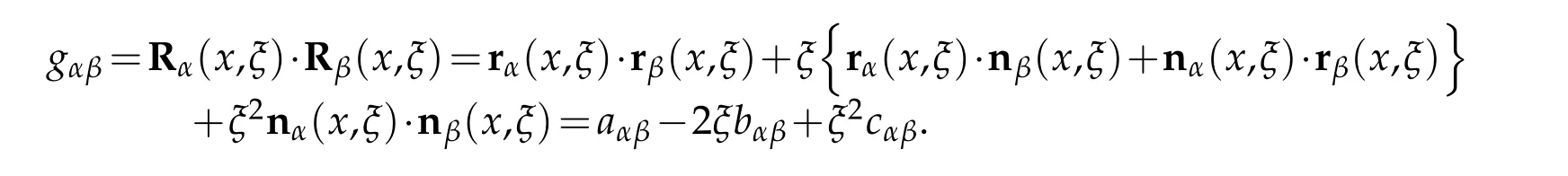
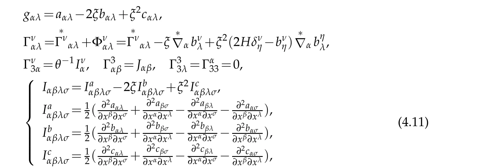
Lemma 2.2.Under semi-geodesic coordinate system,the covariant componentsof metric tensor of 3D Euclidian space E3are the polynomials of two degree with respect transversal variable ξ and can be expressed by means of the first,second and third fundamental form of surfaceℑ:

where

κλ,λ=1,2 are the principle curvatures of ℑ.

Its contravariant componentsare the rational functions of transverse variable ξ and can be expressed by inverse matrices

where x=(x1,x2)and

In particular,gαβadmits a Taylor expansion

Proof.Let ∀(x,ξ)∈E3

and its derivatives

It is obvious that they are independent on Ω.Hence

Combing the first part of(2.9),we derive

Since|n|2=1,nα(x,ξ)·n(x,ξ)=0,we claim

Consider determinant

With(2.8)

it infers

From(2.8)and(2.9)

we obtain

We complete the proof of(2.16).

In order to prove(2.18),we observe

and

Then

Similarly

With(2.21),we have

Using(2.12),we obtain

Making Taylor expansion

gives(2.20).The proof is completed.

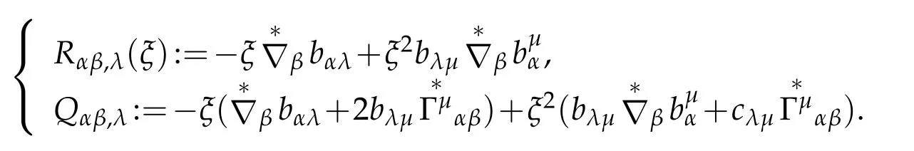
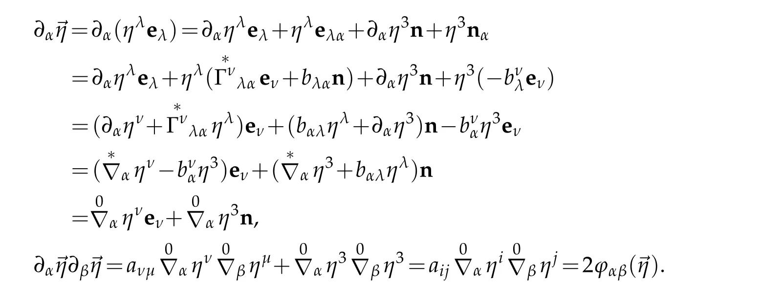
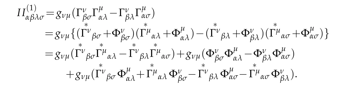
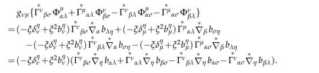
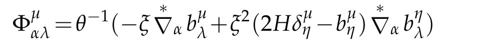
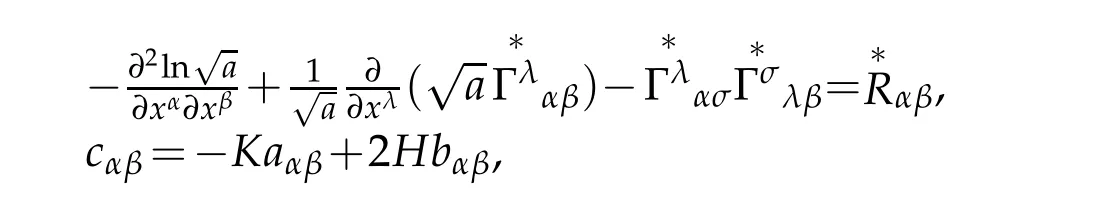
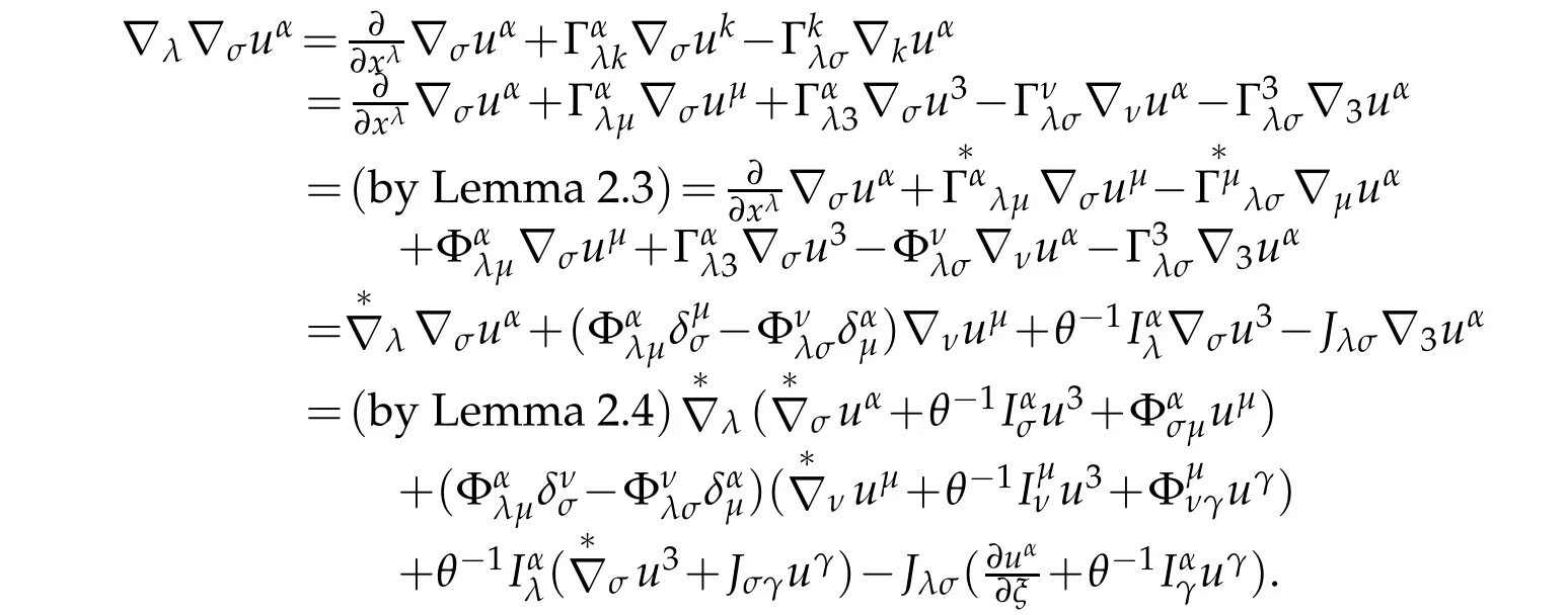
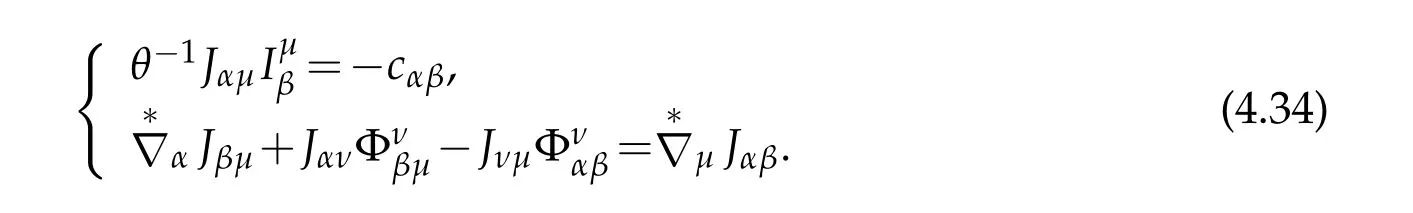
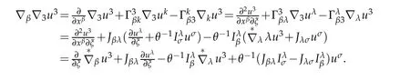
Since ℑ is as a 2D manifold embedded in 3D Euclidian space E3,we need consider the mixed tensor,in particular,mixed covariant derivative for the mixed tensor.Lemmas 2.2 and 2.3 provide the relations between the tensors in E3and those on ℑ.What follows,we consider others relations,for example,let,anddenote Christoffel symbols and covariant derivative in E3and on ℑ respectively,

Then we have

Lemma 2.3.Under S-coordinate system,Christoffel symbolsin E3can be expressed by means of Christoffel symbolsof ℑ

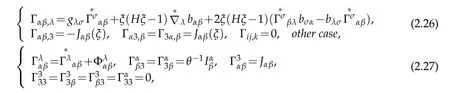
where

Proof.With Weingarten formula and Gaussian formulae

we have

Therefore,

Here we used Gadazzi formula and the covariant derivative of bαβ

where

We complete the proof of first part of(2.26).

Similarly,

Next we prove(2.27).In deed,from the first part of(2.26),we derive

As the covariant derivative of metric tensor is vanished,from Godazzi formula,we have

It can also be expressed by

Taking(2.19)into account,simply computation shows

Therefore,

This is the first part of(2.27).In addition,

Other conclusions can be proved easily.

As we all know,the covariant derivatives of tensor in E3and ℑ are defined by

Since ℑ is embedded into E3,there are relations between covariant derivatives of tensor at different level.

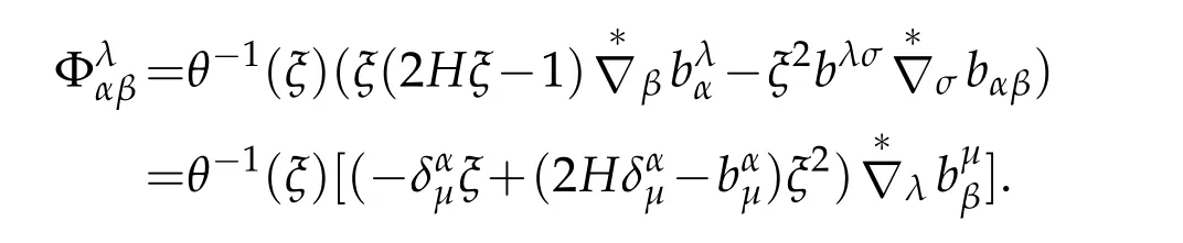
Lemma 2.4.Under S-coordinate system covariant derivative of a vectorin E3can be expressed by derivatives of its components on the tangent space at ℑ.Furthermore it is a rational function of transversal variable ξ

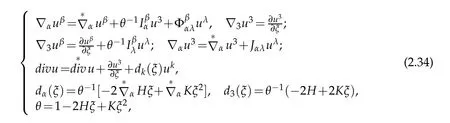
which admit to make Taylor expansion with respect to transversal variable ξ

where

Proof.Note that(2.34)can be easly derived from(2.33)and(2.27).In order to consider Taylor expansion,it is value to mention that when ξ is small enough,function θ-1can be made Taylor expansion

Since

it immediately yields(2.35)and(2.36).Remind that we have to compute divergence.In fact,

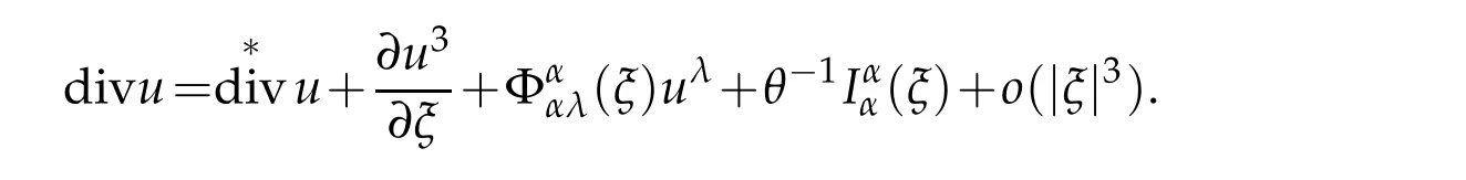
Applying Godazzi formula and Lemma 2.1,

we have

Combining above results,it is easy to obtain(2.35)-(2.37).The proof is completed.

Following lemma is very useful throughout this paper which indicates the relations betweenand so on.

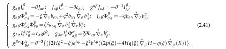
Lemma 2.5.The following formulae are valid

Proof.Repeatedly using Lemma 2.1,we have

Since

we have,

Next,we compute

Since

this follows from the first part of(2.12)that

we obtain

Combining above results we get the forth part of(2.41).

Taking the first and second part of(2.41)into account,

It yields seventh of(2.41)

Next we prove the fifth part of(2.41).Note that

By(2.12)

and θ=1-2Hξ+Kξ2and(2.9)

simple calculation shows that

This is the fifth part of(2.41).

In order to prove the eighth part of(2.41),bywe obtain

Next,we prove sixth of(2.41).Indeed,from fourth of(2.41)it gives that

This is sixth of(2.41).

Finally,we have to prove the night part of(2.41). From(2.18),(2.28)and Godazzi formulait leads to

Therefore,

Since covariant derivative of metric tensor is vanished,from Lemma 2.1,with bβσbβσ=it is not difficult to obtain

Indeed,

but

hence

Finally we obtain

The proof is completed.

In what follows,we consider strain tensor eij(u)in E3associated with displacement vector u

We use derivative of metric tensor being vanished

which will be frequently used throughout this paper.

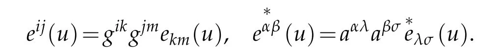
The contravariant component of vector u:uk=gkjujinstead of covariant component of vector.The strain tensor on ℑ associated with displacement vector u:

The contravariant components of strain tensor are defined by

We also consider Green St.Vennant strain tensor Eij(u)of the displacement u for nonlinear elastic case

Lemma 2.6.Under S-coordinate system the strain tensor and Green St.Vennant strain tensor are the polynomials of degree two with respect to transverse variable ξ

where

where the strain tensors on the two-dimensional manifold S are given as:

where

Remark 2.1.Since displacement vector u3=0 andat tangent space of 2D manifoldℑ,the strain tensor is given bywhile displacement vector are in 3D space,the strain tensor of displacement vector restrict on the ℑ will be given by γαβ(u).

Proof.

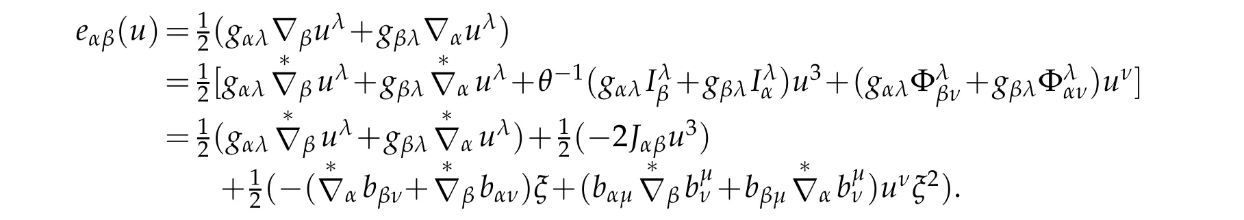
Since of Godazzi formula and vanishing of covariant derivatives of metric tensor,we get

Next,we prove the second part of(2.46).With(2.41)and Godazzi formula,we have

It infers that

In what follows,we prove

Indeed,by(2.28)we derive

Taking into account of

and(2.54),we immediately obtain our conclusion.By above discussion,it infers that

where

with

Applying(2.36)immediately derive formula(2.50).

By similar manner,the Calculations show that

where

Furthermore,from(2.4)and(2.34)we have

where

Our proof is completed.

We assume that the elastic material constituting the shell are isotropic and homogenous.The contravariant components of elasticity tensor are given by

where(λ≥0,µ＞0)are the elastic coefficient constants.Let

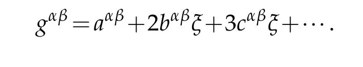
Lemma 2.7.The elasticity tensor are a rational polynomials with respect to ξ in the S-coordinate system:

where

Proof.From(2.55)and(2.18),simple calculation show our results.The proof is complete.

In what follows,we introduce following invariant scale function

3 The metric tensors after deformation of the surface in ℜ3

In this section,we have to study the exchange of geometry of the surface in ℜ3when the surface occurs deformation.We will give the formula for the exchange of metric tensor,curvatures tensor and normal vector to the surface.

Let ω ⊂ℜ2be a compact domain and a immersionis smooth enough,the middle surface ℑ of shell defined as the imageThe deformation of a surface means that at each point on the surface bears a small displacement →η and new surface after deformation denote ℑ(→η)as the image

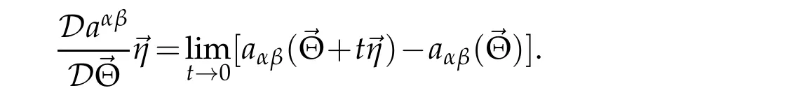
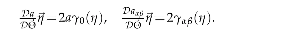
For simplicity,later on,we denote the Gateaux derivative of a geometric tensor(for example,metric tensor)with respect to surface →Θ along director →η

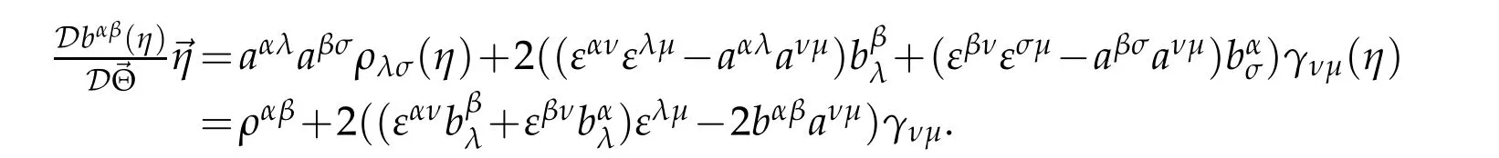
Theorem 3.1.Assume that surface ℑ is burned a deformationThen following formulae hold

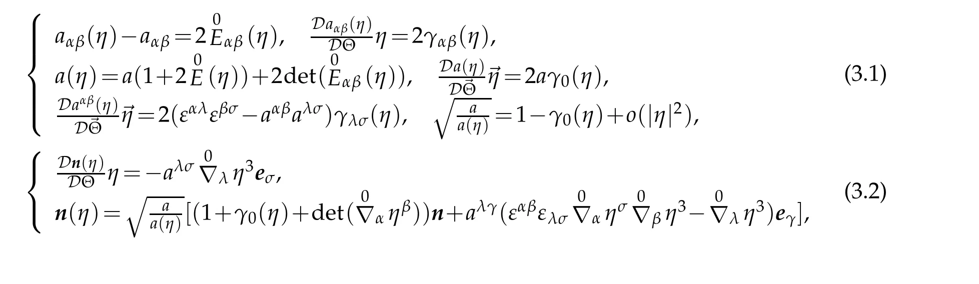
The Gateaux derivative of Riemann curvature with respect to surface ℑ along direction →η is given by

where

Proof.(i)Preliminary

Assume that the displacement vector and base vectors of S-coordinate system at ℑ

are given.Then

Proposition 3.1.The followings on the ℑ are valid

Proof.Indeed,using Gaussian and Weingarten’s formula,reads

From above formula(3.7)is obtained.

What follows that we prove(3.8),In fact,by virtue of Weingarten’s and Gaussian formula

and(see[2])

Therefore,

Observe that

Taking into account of

from(3.11)it infers(3.8)immediately.

(ii)Metric tensor and its determinanta(η)=det(aαβ(η)).

Proposition 3.2.The Gateaux derivatives for metric tensors and its determinant with respect to ℑ along director →η are given by the followings

Furthermore,

Proof.The deformed surface ℑ(η)define as the imageAssume vectors

are linearly independent at all points ofIt is obvious that if the vectoris small enough,e(η)can be as base vectors of two dimensional manifold ℑ(η).So that aαβ(η)=eα(η)eβ(η)are covariant components of metric tensor of ℑ(η)which is nonsingular matrix.Indeed

By(3.7),

According to the calculation’s principle of the determinant for a matrix

and the formula

we assert

Therefor there exist contravariant components of metric tensor

where the permutation tensor is defined by

Let the normal unite vector be

and the contravariant base vector

From this,of course,it infers

The second and third terms of the above equality are two degree of η,so that with(3.13)

On the other hand

The proof of Proposition 3.2 is complete.

(iii)Second fundamental form and unit normal vector n(η)to ℑ(η)

Proposition 3.3.The Gateaux derivatives for unit normal vector with respect to ℑ along director →η are given by the followings

From(3.7),(3.10)and the formula

it infers

Here we used formula

In a similar manner,using(3.8)gives

Substituting above equalities into(3.15)leads to sixth formula of(3.14).

Using sixth formula of(3.14),

Hence we assert

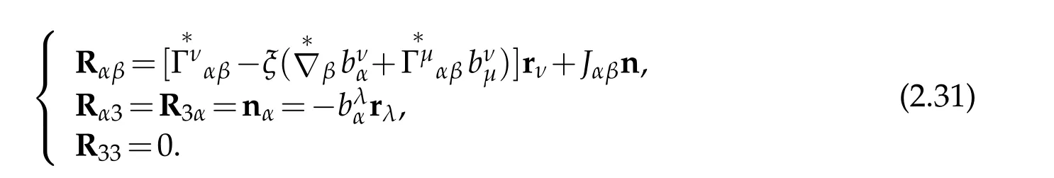
Proposition 3.4.The Gateaux derivatives for curvature tensors and its determinant with respect to ℑ along director →η are given by the followings

where the tensors of order two are defined by

Proof.According to the Gaussian formula

we have

On the other hand,the following formula is held

Indeed,by the Weingarten’s and Gaussian formula(3.9)

Hence,we conclude(3.19)by virtue of(3.17).Using the Weingarten’s formula(3.9)with(3.19),we assert

Coming back(3.18)with(3.7)and(3.9)shows

It can be rewritten in

These are the first second of(3.16).Next we consider the contravariant component

Using above,(3.12)and(3.16),and link chain of derivative

Note that

If b=det(bαβ)/0 then

Hence

To sum up,it completes our proof.

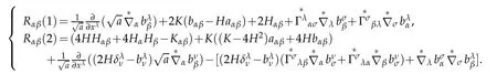
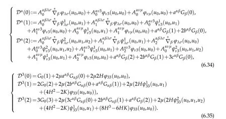
Proposition 3.5.The Gateaux derivatives for(H,K,cαβ)with respect to ℑ along director→η are given by the followings

Proposition 3.6.The Gateaux derivative of Riemannian curvature tensor with respect to surface ℑ(η)is give by

Indeed,the Riemannian curvature tensor of surface ℑ(η)is given by

Applying Proposition 3.4 immediately yields to(3.21).

(iv)Symmetry of indices forραβ(η)and(η)

Let us define the tensor ραβ(η)of order two and(η)of order three generated by the displacement vector

Proposition 3.7.The tensors ραβ(η)and(η)are symmetric tensors with respect to index(α,β):

and have equivalent form

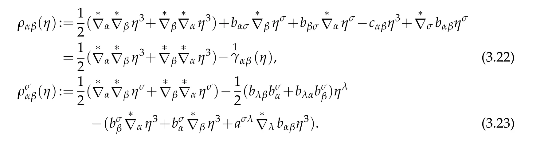
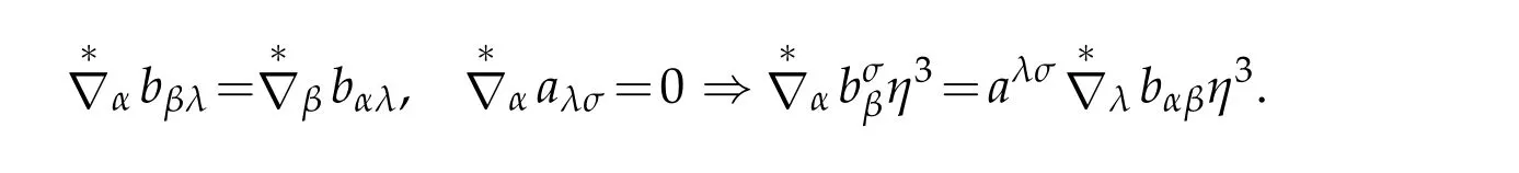
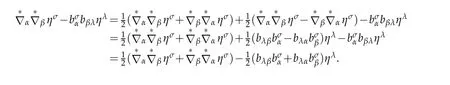
Proof.First,we prove(3.22)and(3.23).Indeed,by virtue of(2.36)and(3.17),

since η3is looked as a scale function define on ℑ and Goddazi formula we claim

From this and(2.47),it implies(3.22).Next we prove(3.23).In fact,by(2.29),we claim

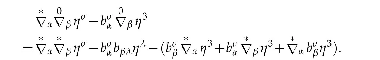
Since the Godazzi formula and the covariant derivative of metric tensor being vanishing,

In addition,by virtue of the Ricci formula

Hence

Finally,we end our proof for Theorem 3.1.

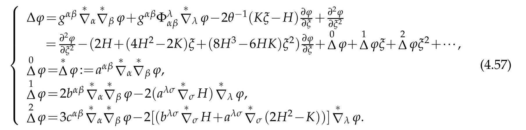
4 Differential operator in the S-coordinate system

Hoge-Laplave operator under S-coordinate system

It is well known that for the Navier-Stokes equations in fluid mechanics or the Lamee-Navier equations in elastic mechanics,their principle part contain the divergence of the strain tensor for velocity vector or displacement vector.In the Riemannian space,they do not have interchangeability with Leray projector on the divergence free subspace Kerdiv,but it is possible to make interchange with the Hoge-Laplave operator.In order to make mix with either self,denote ΔHby

where d and δ are the exterior differential operator and the supper differential operator,respectively.According to the Weitzenbock formula,it is equal to Bochner-Laplace(traci-Laplace)plus Ricci operator when it acts on vector field,i.e

where Bochner-Laplace operator is defined by

It is well known that the conservation of the energy-momentum in physics concern divergence of enrgy-momentum tensor,the constitutive equation in continuum also contain the relationship between strain tensor and stress tensor.It is natural that the divergence of strain tensor play important role. The relationship of strain tensor,Bochner-Lpalace operator and Ricci operator in Riemannian space are given by

Combining above notations,the divergence of the strain tensor in higher space and two dimensional surface are given by

respectively. It is obvious that it is enough to compute the Bochner-Laplace operator when we have to compute the divergence of strain tensor.

By the way in 3D-Euclidean space E3,following is given in terms of the operator rotrot to compute divergence of strain tensor

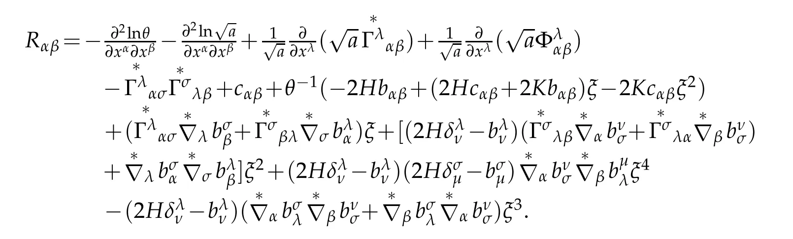
The following theorem gives the expansion with respect to the transverse variable ξ for the Riemmannian curvature and the Ricci curvature tensors.

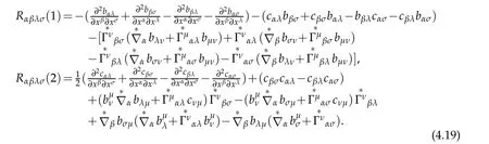
Theorem 4.1.Under S-coordinate in the 3D-Riemmannian space,the Riemannian curvature tensor is a polynomial of degree two with respect to the transverse variable ξ

where

Proof.At the first,we give the expression for the Riemann curvature tensor of four order covariant components under S-coordinate.To do that,according to

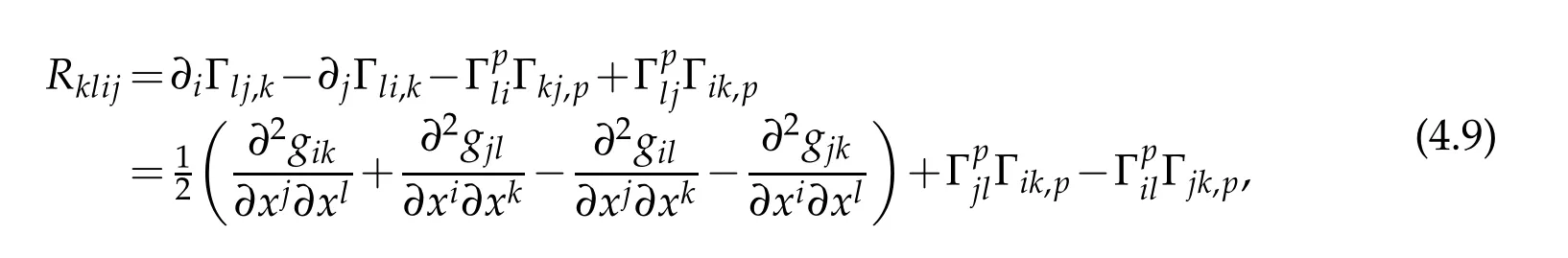
and(2.16)-(2.17),we have

By applying

we have

According to the formula for the Riemann curvature in 2D Surface([1])

Therefore

By appling(2.27)and(2.28)

it yields

Using

and(4.14),we have

where we have used the following two equalities

Finally,

it still possess anti-symmetric of indices.Combing(4.14)and(4.15)with(4.12)yields

Substituting(4.11),(4.12)and(4.16)into(4.9)leads to

Owing to the anti-symmetric of index of Riemann curvature tensor

the sum of first three terms in(4.17)equal to zero

Then(4.17)becomes

It can be also expressed by

Let us define a tensor of four order covariant components

Then(4.17)becomes

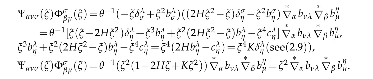
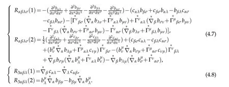
The remaining is to prove formula(4.8)

Using

and the Godazzi formula

we obtain

On the other hand,by(2.41)

Substituting into(4.24)leads to

Combining(4.22),(4.24)and(4.25)yields

By symmetry and anti-symmetry of indices for Rimemann curture tensor,we obtain

In what follows,

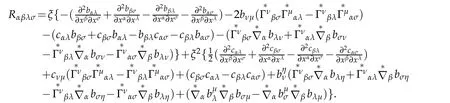
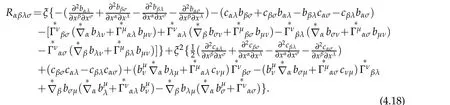
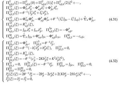
Theorem 4.2.Under the S-coordinate in the 3D-Riemmannian space,the Ricci curvature tensor is a rational polynomial of degree two with respect to the transverse variable ξ whose Taylor expansion is given by

where Hα=∂αH,

Proof.Applying Lemmas 2.2,2.3 and 2.5,and g=θ2a,we have

On the other hand,

Similarly,

Note that

we have

Furthermore,

Thanks to

Finally

In addition

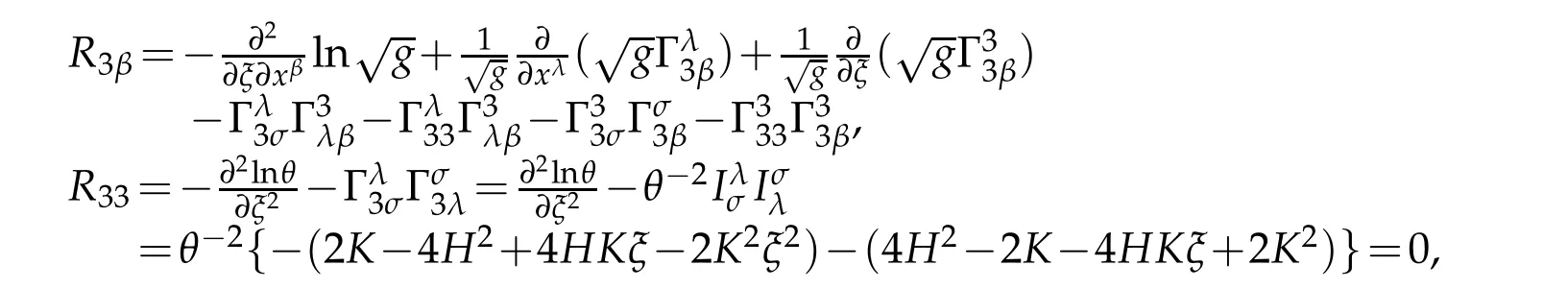
It follows from

that

Since

we obtain

The proof is complete.

Next we consider the relationships of covariant derivatives of order two in 3D-space and on the two dimensional manifolds which are necessary for studying differential operators on the manifolds.

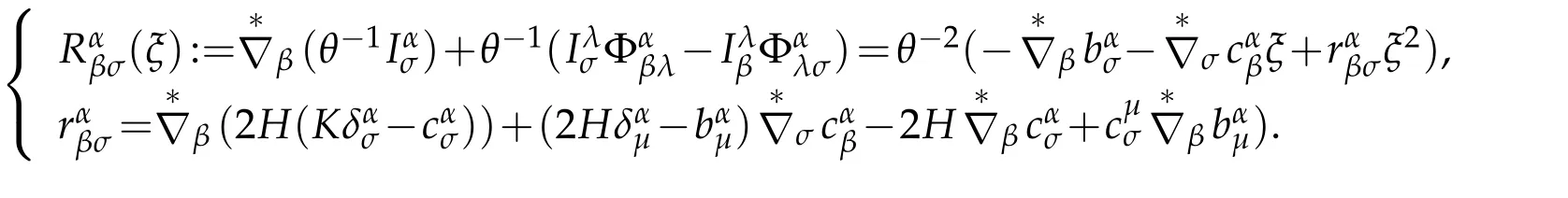
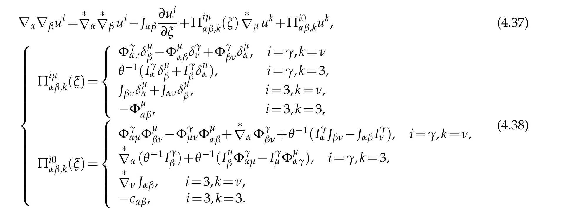
Lemma 4.1.There are relationships between the covariant derivatives of two order of the vectors in 3D space and on two dimensional manifold

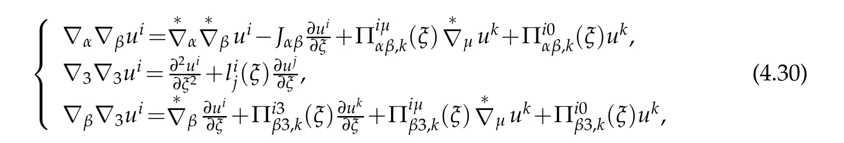
where

and

Proof.In order to prove Lemma 4.1,we repeatedly and alternately to apply Lemmas 2.1-2.7.Indeed,for example,according to the definition of covariant derivative of second order tensor

Making rearrangement to obtain

Next we consider

Below we prove

In fact,in view of(2.41)

In addition,we have

Using the Godazzi formula

we assert

Substituting above formula into(4.35)leads to

From this it yields(4.34).Finally we obtain

Combing(4.33)and(4.36)we claim

Next we consider

Owing to(2.27):

it infers

The following equality is very useful later on

To obtain that,we first show that

On the other hand,

so that

This infers(4.41).Coming back to(4.40)

In addition,in view of(4.39)we have

Combining(4.42)and(4.43)gives

Next we compute

Finally we find

Straightforward calculasions show

Howerver

Therefore

On the other hand

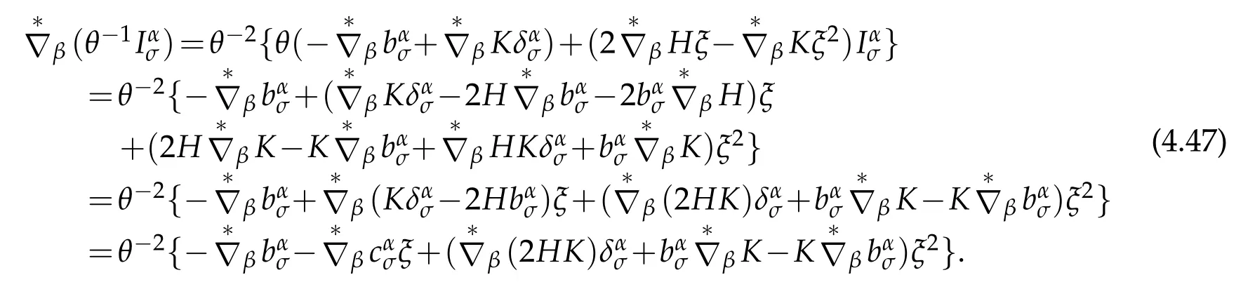
Combining(4.46)and(4.47)leads to

Owing to

and applying(4.46),(4.45)becomes

By a similar manner,we find

Note that

we have

With(4.45)we assert

where

To sum up we verify(4.30).

Theorem 4.3.Under the S-coordinate system in the 3D Riemannian space,the Bochner-Lplace operator acting on a vector field can be expressed in a rational polynomial with respect to the transverse variable(the length of geodesic curve)ξ.

where

Remark 4.1.The Taylor expansions in(4.53)are given by

Proof.Applying Lemma 2.2 and Lemma 4.1

By virtue(4.31)and Lemma 2.5

Applying(4.46)and Lemma 2.1it yield

Hence,we obtain the 2nd and 3rd parts of(4.53).

Theorem 4.4.Under the S-cooedinate system in the 3D Riemann space,the Betrimi-Laplace operator Δ=gij∇i∇jis a polynomial with respect to transfers variable ξ,which can be made Taylor expansion with respect to ξ,i.e.for a two times differential function φ,

Proof.Indeed,by(2.34),

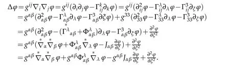
Since

it is not difficult to prove that

Therefore

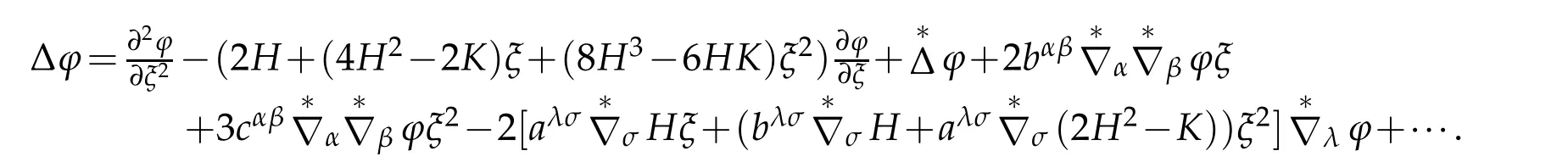
The proof is completed.

5 A dimensional splitting form for linearly elastic equations in 3D shell in ℜ3

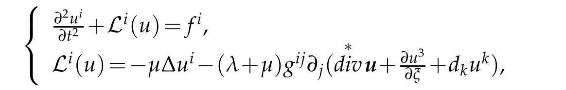
As well know that the initial and boundary value problem of linearly elastic mechanics are give by

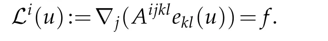
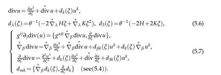
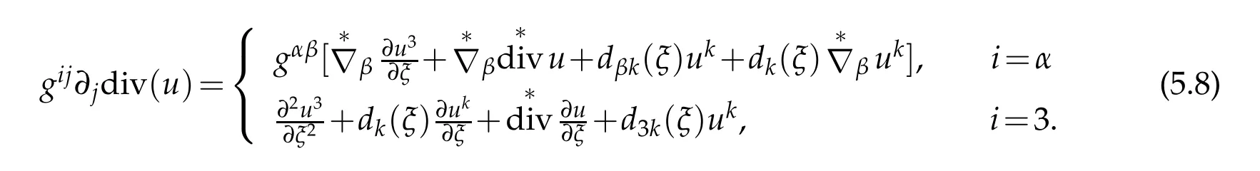
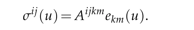
Since Aijklis defined by(2.55)and gklekl(u)=divu,we claim

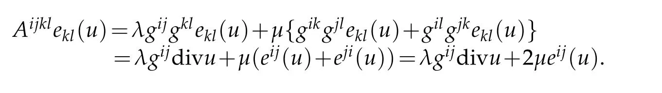
Therefore

Applying the Ricci formula

if E3is Euclidian space,Furthermore

where Rmkare Ricci curvature tensor.

In this case,the linear elasticity operator is given by

Finally elasticity equations in Euclidian space are given by

where the lateral surface Γ0=Γ01∪Γ02,σ is a stress tensor.

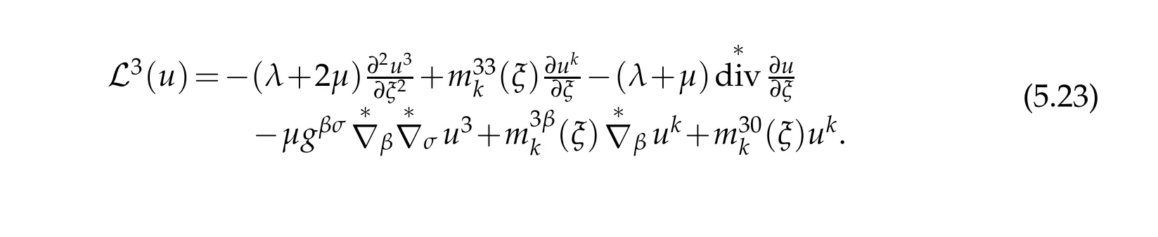
Theorem 5.1.Under the S-coordinate system in E3,Eq.(5.1)can be expressed as

in details,

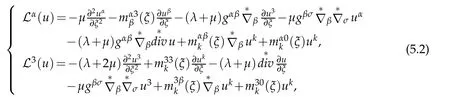
where

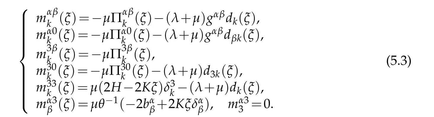
Matrices dijare given by

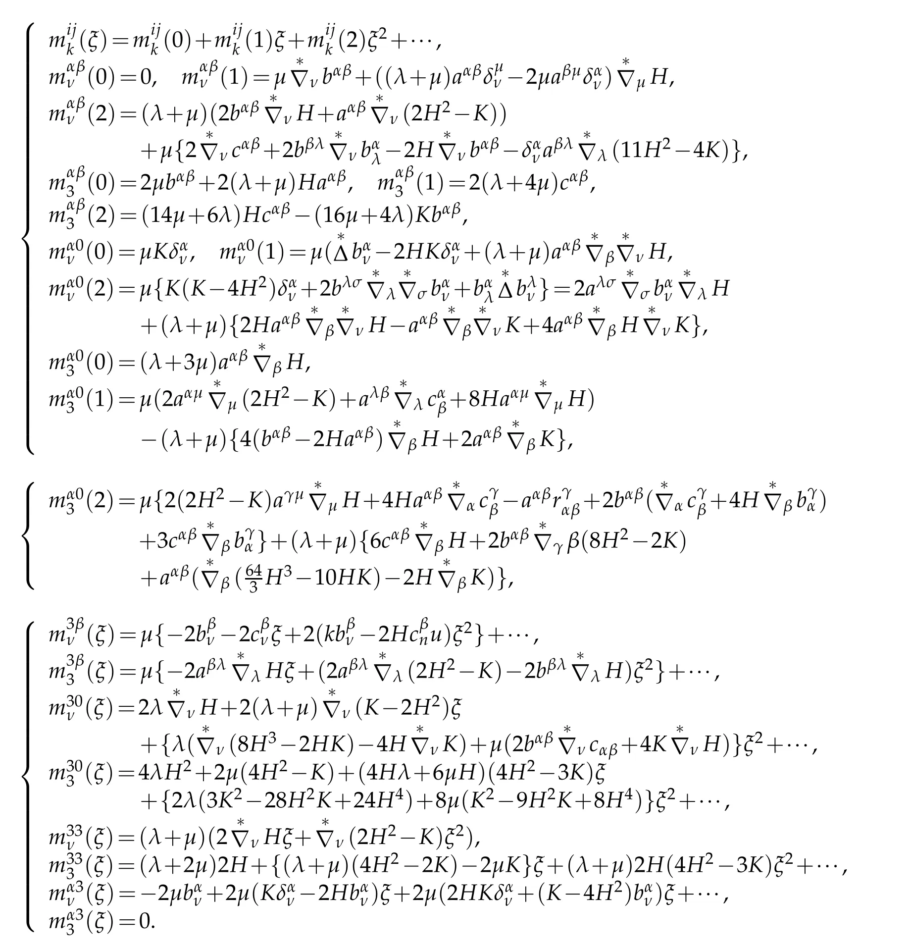
Remark 5.1.Taylor expansions of(5.3)are given by

Proof.At first we prove(5.2).To do that,since(4.30)and(2.35),rewritten(5.1)into components form

In addition,

Therefore

Substituting(5.6)leads to(5.2),we end our proof.

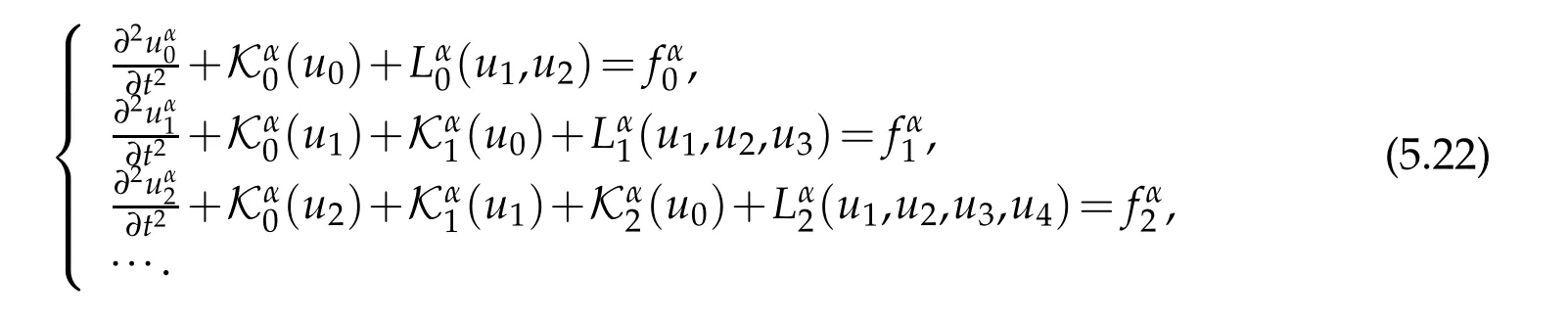
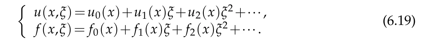
Theorem 5.2.Under the S-coordinate system in E3,if the solution of(5.1)in neighborhood of surface ℑ and right hand f can be made Taylor expansions with respect to transverse variable ξ

then the linear elasticity operators cam be made Taylor expansions as

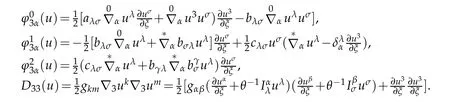
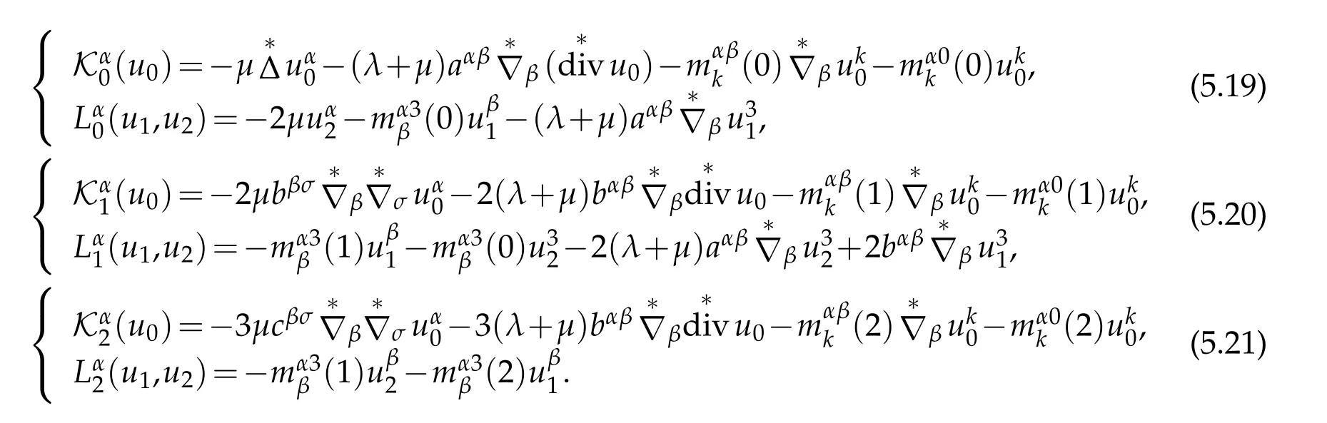
where u0(x),u1(x),u2(x)satisfy following boundary value problems

with boundary conditions in(5.1)on the boundary γ1=Γ02∩{ξ=0}of middle surface

where

Proof.Consider(5.2)

Using

gives

Denote

Taking(5.18)-(5.21)into account,(5.17)can be made expansion

So that we obtain following equations

By similar manner,we assert

Substituting(5.10)into(5.23)leads to

Hence it can be expressed as

Consequently,we obtain following equations

where

We then complete our proof.

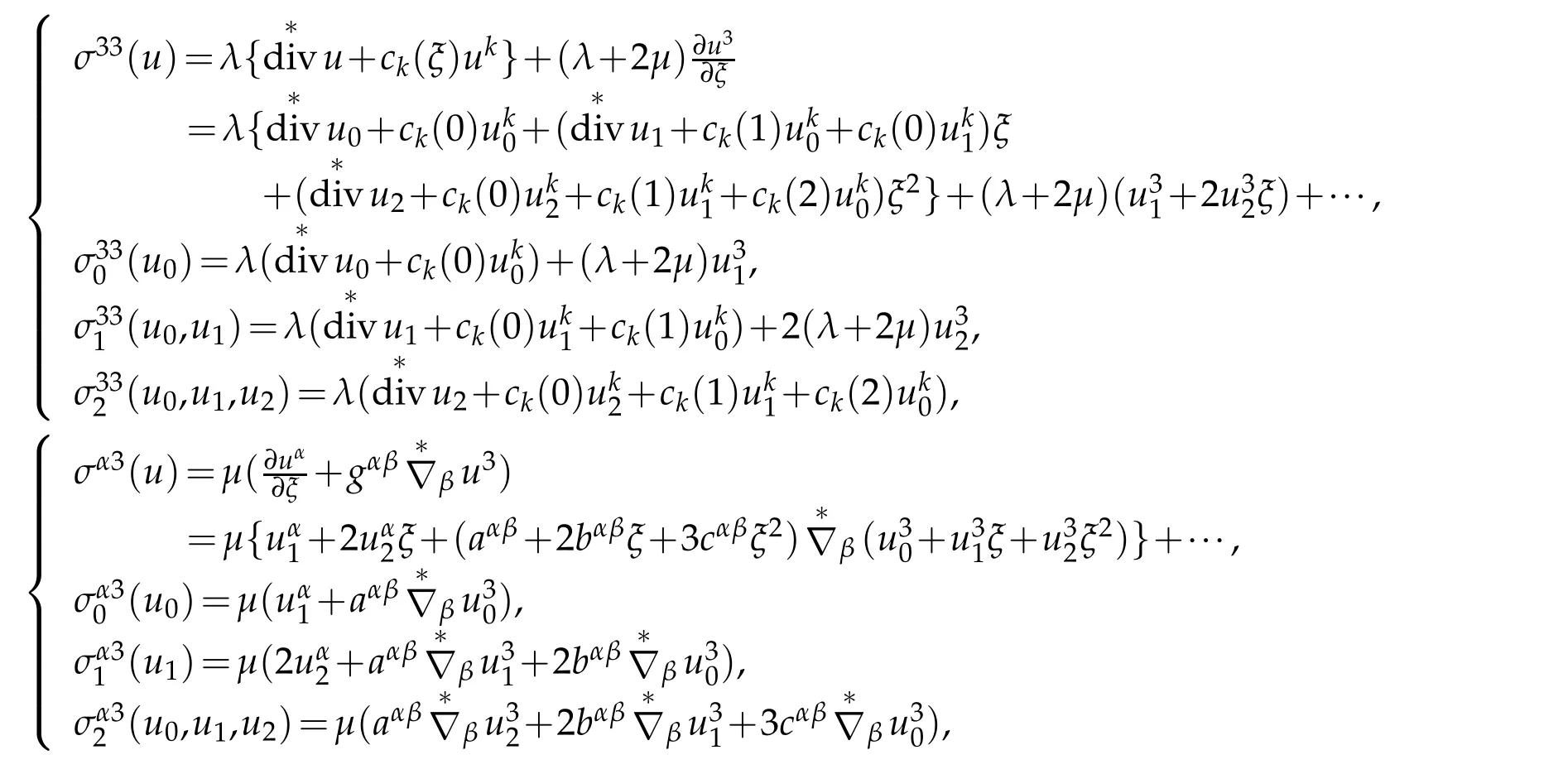
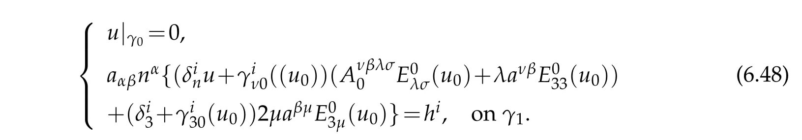
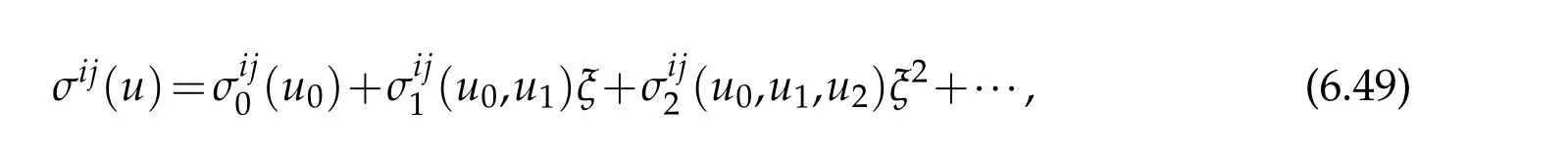
Theorem 5.3.Under S-coordinate system in E3,if(5.5)is satisfied then linearly stress tensor σij(u)=Aijklekl(u)can be made Taylor expansion with respect to transverse variable ξ

where

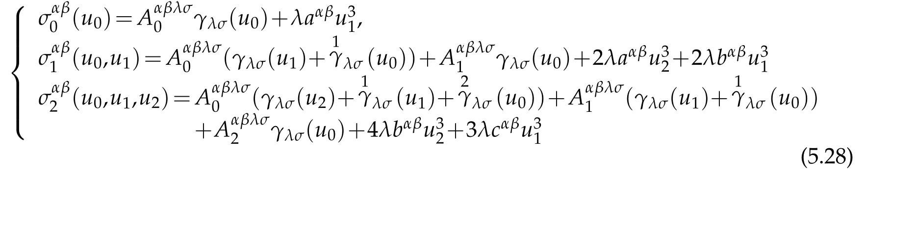
where

The boundary conditions on top and bottom surface of shell are given by

Proof.As well known that linearly stress tensor σij(u)of isotropic linearly elastic materials corresponding to displacement vector u is given by

Elastic coefficient tensor of isotropic linearly elastic materials is given by(2.55)and can be made Taylor expansion with respect to transverse variable ξ by(2.57). In addition,owing to Lemma 2.6 andare linear form for u,therefore

Note non vanishing Aijkmby Lemma 2.7

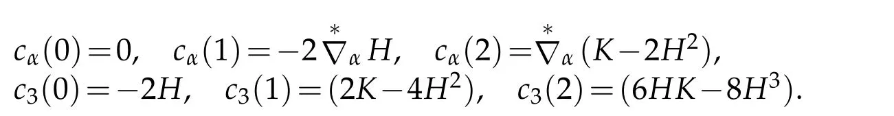
where ck(ξ)defined by(2.34).Thanks to(2.20)

We assert that

From this it yields(5.29).Moreover

where ck(ξ)are defined by(2.34)

Hence

Finally,boundary conditions on the top and bottom of shell are nature boundary conditions

Note,in Theorem 3.1,displacement →η=ε→n=(0,0,1)at top surface of shell,it yields from(3.2)

Therefore,by Theorem 5.2,we have

Similarly,since n(-εn)=-n,hi=gjmσij(u)nm(-εn)on the bottom surface of shell,so that

This completes our proof.

6 A dimensional splitting form for nonlinearly elastic equations in 3D shell in ℜ3

In this section we study nonlinearly elastic equations for isomeric and isomorphic St.Venant-Kirchhoff materials.Nonlinearly elastic equations for 3D elastic shell are given by:findsuch that:

where stress tensor σij,second Piola-Kirchhoff stress tensor Σijand first Piola-Kirchhoff stress tensorare given respectively by:

where eij(u),Eij(u)are strain tensor(2.42)and Green-St Venant strain tensor(2.45).

In the followings,we have to consider first Piola-Kirchhoff stress tensor.The covariant derivatives of first Piola-Kirchhoff stress tensor are given by

where we consider the materials are isomeric and isomorphic,and covariant derivatives of metric tensor in Euclisean space are vanising(i.e.∇jAkjlm=0).As well known that linearly elastic operator

Therefore nonlinearly elastic operator is given by

As well known that isotropic and homogenous elstic coefficient tensor of four order are given by(2.55)and satisfiy(2.57),in particular all components Aijlmare vanissh except

In addition

So that it assert that

It can be reads as

According Ricci Theorem and Riemannian Curvature tensor are vanish in Euclidian space,therefore

and symmetry of indices of strain tensor,previous equality becomes

Substitute it into(6.5)leads to

Since

Hence

Reads otherwise

Furthermore,by similar manner,we assert

Substitutin it into(6.7)leads to

Next we need to consider relationship of covariant derivatives of nonlinear stain tensor tensor.

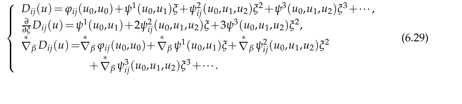
Lemma 6.1.The covariant derivatives of symmetric tensor of stain tensor Dijin S-coordinate system are given by

where

Proof.According to definition of covariant derivative,

By virtue of Lemma 2.3

Therefore,since symmetry with respect to subscript of Dij=Dji,

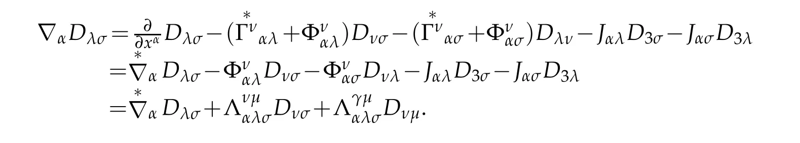
In similar manner,by Lemma 2.3

Other equalities of(6.9)can be obtain in same way.End our proof.

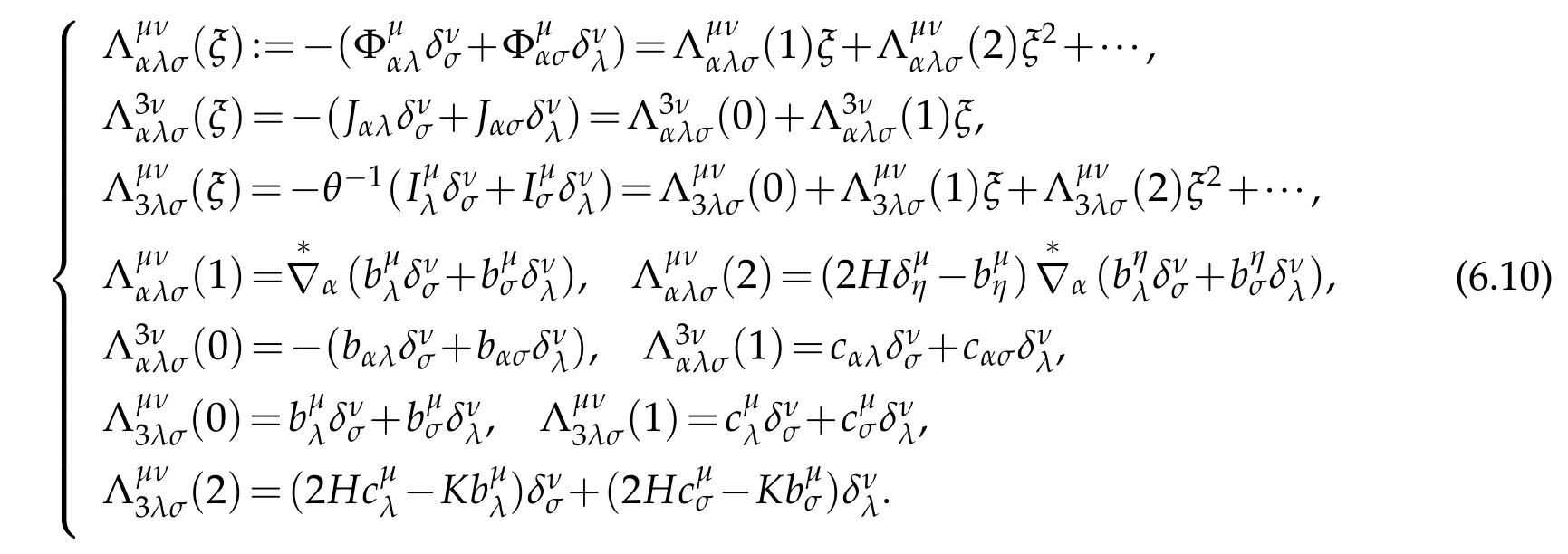
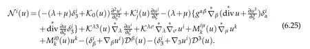
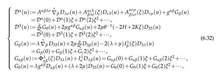
Lemma 6.2.Assume that the elastic materials is isomeric and isomorphic St.Venaut-Kirchhoff materials. Then under S-coordinate system nonlinear elastic operator defined by(6.1)can be expressed as

where Eij(u)is Green-St-Vennant strain tensor defined by(2.45)and

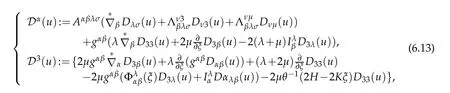
Proof.Taking(6.9)into account,we claim

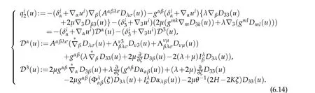
Similarly,applying Lemma 4.1 and Theorem 4.3 and Theorem 5.1,we assert

where

Owing to(5.2)

with(6.8),(6.14)and(6.15),we obtain

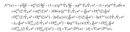
which can be rewritten as

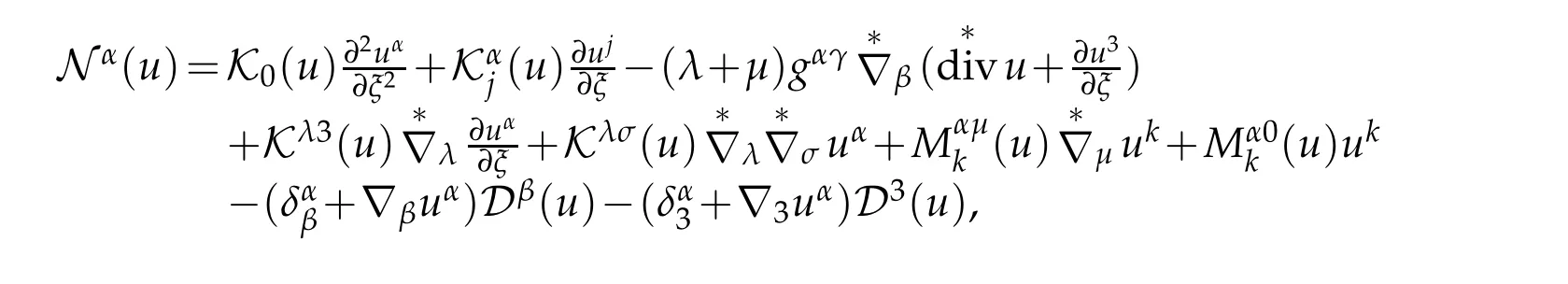
where

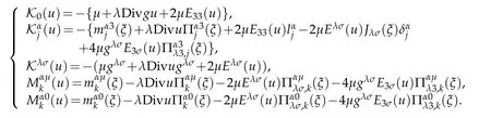
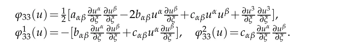
Third component is given by

which also can be expressed as

where

To sum up,nonlinearly elasticity operators can be written as

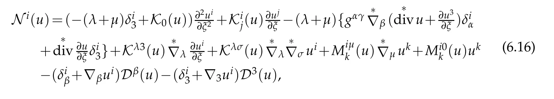
where

Hence we complete our proof.

Theorem 6.1.Assume that solution u of nonlinearly elastic operators defined by(6.11)and right hand term f can be made Taylor expansion with respect to ξ:

Then nonlinearly elastic operators defined by(6.11)under the S-coordinates can be made Taylor expansion

and(u0,u1,u2)satisfy approximately following boundary value problems

with boundary conditions

where

Proof.As well known that the nonlinearly elastic operators are given by(6.11),

As well known all coefficients can be made Taylor expansions with respect to transverse variable ξ if taking(6.19)into account

Therefore

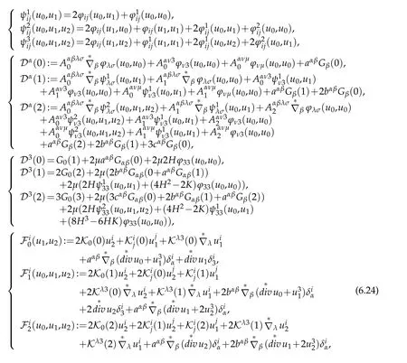
Next we consider Didefined by(6.18).To do that let remember bilinear and symmetric form D(u)defined by(2.48)

Denot e

The n

In addition,let

Then

Let us come back to(6.18).Note that

where

Futhermore,in view of(2.34)and(6.19)we claim

where

Owing to(6.36)and(6.32)we assert

Substituting(6.38)and(6.26)into(6.25)leads to

This is(6.20).

Next we consider expansion for bilinearly symmetric form. Note Green St-vennen strain tensor Eij(u)of vector u is defined by(2.45)

and satisfies following formula(see Lemma 2.6)

which are polynomials of two degree with respect to transverse varialble ξ,and its coefficients do not contain three dimensional cavariant derivativesof displacement vector u but contain two dimensional derivativeson the surface.Therefore if displacement vector satisfies Taylor expansion(6.19),then we claim

Let us denote

where

Finally,the coefficients in(6.26)are given by using(6.12),(6.41),(6.42)and(6.44).

Next we have to give boundary conditions

where σ are the first Piola-Kirchhoff stress defined by(6.2)

The normal vector n on γ1is n-nαeα,

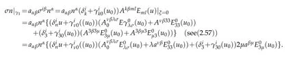
Hence boundary conditions are given by

The proof is completed.

Theorem 6.2.Assume that solution u of nonlinearly elastic operators defined by(6.11)and right hand term f can be made Taylor expansion with respect to ξ(6.19).Then the first Piola-Kirchhoff stress

defined by(6.2)on ℑ under the S-coordinates can be made Taylor expansion

where

Proof.As well known that according to(6.2)the first Piola Kirchhoff stress tensor are given by

Then using(2.57),(6.51)and(6.52)we can obtain Taylor expansion for σij. By similar manner we also can obtain for other expansions.The proof is completed.

7 An Example:Hemi-ellipsoid shell

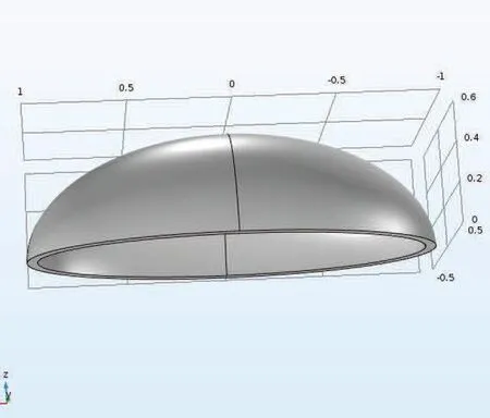
Let us consider the hemi ellipsoid shell.As well known that parametric equation of the ellipsoid be given by

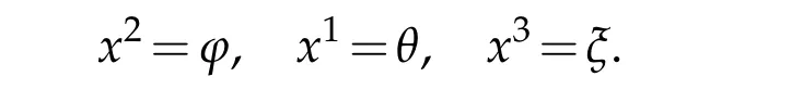
where(i,j,k)are Cartesian basis,(φ,θ)are the parameters and(x1=φ,x2=θ)are called Guassian coordinates of ellipsoid.The base vectors on the ellipsoid

The metric tensor of the ellipsoid is given by

Owing to

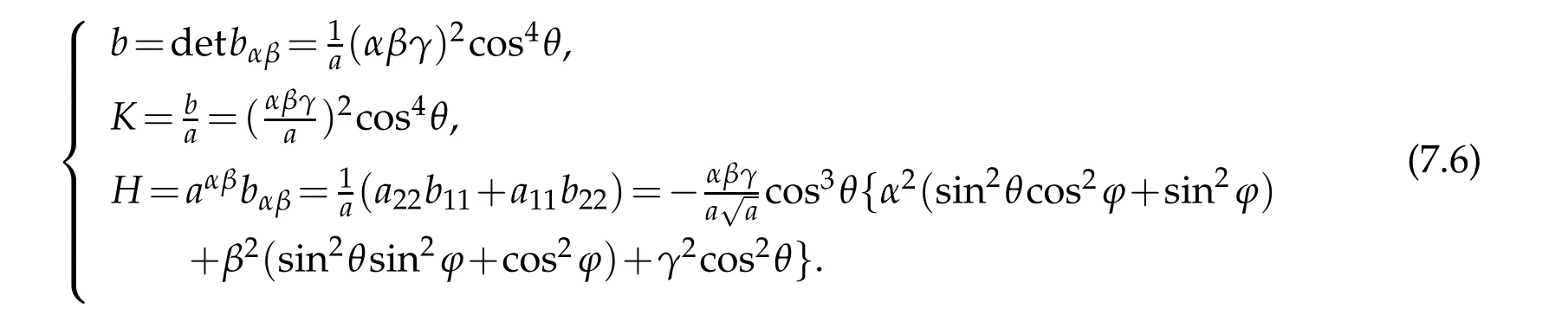
the coefficients of second fundamental form,i.e.curvature tensor of ellipsoid

Consequently,curvature tensor,mean curvature and Gaussian curvature are given by

Semi-Geodesic coordinate system based on ellipsoid ℑ

Note that

The radial vector at any point in ℜ3

We remainder to give the covariant derivatives of the velocity field,Laplace-Betrami operator and trac-Laplace operator.To do this we have to give the first and second kind of Christoffel symbols on the ellipsoid ℑ as a two dimensional manifolds

Then covariant derivatives of vector u=uαeα+u3n on the two dimensional manifold ℑ

As well known that displacement vector u=(u1,u2,u3)on middle surface of shell has three components,third component u3looked as scale function,is a Laplace-Betrami operator on ℑ which is given by

The trace-Laplace operatoe on ℑ is given by

Next let return to stationary equations(5.6)with boundary value

and consider associate variational formulations for(u,u1),find(,i=1,2,3)∈(ω)3×(ω)3,such that

Note that(5.13)shows that

Note that integrals by applying the Gaussian theorem become

Let us denote

By similar manner

In addition,

Therefore,we assert

The variational problem(7.13)can be rewritten as,findsuch that

Taking(7.5),(7.15)and Remark 5.1 into account,simple calculations show that

Substituting(7.22)into(7.18)and(7.20)leads to

The bilinear form of the variational problem(7.21)is given.

Acknowledgements

This research was supported by the National Natural Science Foundation of China(NSFC)(NO.11571275,11572244)and by the Natural Science Foundation of Shaanxi Province(NO.2018JM1014).