
Couple stress fluid flow in a rotating channel with peristalsis *
2018-05-14 01:43AbdelmaboudSaraAbdelsalamKhMekheimer
水动力学研究与进展 B辑 2018年2期
Y. Abd elmaboud , Sara I. Abdelsalam , Kh. S. Mekheimer
1. Mathematics Department, Faculty of Science and Arts, Khulais, University Of Jeddah, Jeddah, Saudi Arabia.
2. Mathematics Department, Faculty of Science, Al-Azhar University, Cairo, Egypt
3. Department of Mechanical Engineering, University of California, Riverside, USA
4. Mathematics Department, Faculty of Science, Al-Azhar University (Assiut Branch), Assiut, Egypt
5. Basic Science Department, Faculty of Engineering, The British University in Egypt, Cairo, Egypt
Introduction
The theory of the couple stress (CS) fluid was first proposed by Stokes[1]in 1966. In this theory Stokes introduced the rotational field in terms of the velocity field for setting up the constitutive relationship between the stress and strain rates. Stokes microcontinuum theory allows for polar effects such as the presence of couple stresses, body couples and a nonsymmetric stress tensor.
Peristaltic transport is one of the important topics that attracts scientific researchers in bio fluid mechanics branch. Peristaltic transport is a physical mechanism for the flow induced by the traveling wave. This mechanism is found in the body of living creatures,and it frequently occurs in organs such as ureter,intestines and arterioles (small arteries). The mechanism of peristaltic transport has also been found in the industry. There are many industrial applications that involve peristaltic transport, some of which, sanitary fluid transport, blood pumps in heart lung machine,and transport of corrosive fluids where the contact of the fluid with the machinery parts is prohibited. The first investigation of peristaltic transport was done by Latham[2]. Recently, considerable attention has been devoted to the problem of peristaltic transport with Newtonian or non-Newtonian fluid in channel or a tube[3-16].
In most mathematical models there are some difficulties to achieve the exact solution. Homotopy analysis method (HAM) ( homotopy perturbation method (HPM) is a special case) is a new analytical technique that employs a transformation procedure which reduces the involved partial differential equations into ordinary differential equations. Series solutions of the resulting systems are constructed. The convergence of the obtained series solutions is seen through graphical results and tabular values. The method gives flexibility in the choice of basic functions for the solution and for the linear inversion operators (when compared with the Adomian decomposition method), while still retaining a simplicity that makes the method easily understandable from the standpoint of general perturbation methods. This method has been first introduced by Liao[17,18].Recently, many authors[19-22]have used HPM in a wide variety of scientific and engineering applications.
Motivated by these ideas, the goal of this investigation is to study the couple stress fluid flow in a rotating channel with peristalsis. The governing equations are modeled and reduced to a simple form using the long wavelength approximation then solved using the HPM. The analyses for the velocity, pressure gradient, flow rate due to secondary velocity, and the pressure rise have been discussed for various values of the problem parameters.
1. Formulation of the problem and mathematical model
Consider a two-dimensional infinite channel filled with homogeneous incompressible couple stress fluid. We assume that the channel rotates with a constant angular speed Ω, about theZ′-axis. The flow is induced by sinusoidal wave trains propagating with constant speedc, along the channel walls (see Fig.1). The geometry of the wall surface is defined as

whereais the half-width of the channel,bis the wave amplitude, λ is the wavelength andt′ is the time. With regard to the rotating frame the fluid velocity vector is given byV′= (U′(X′,Z′,t′),V′(X′,Z′,t′),W′(X′,Z′,t′)), whereU′,V′ andW′ are the velocity components inX′,Y′ andZ′, respectively. Introducing the wave frame (x′,y′,z′) that moves with velocitycaway from the fixed frame(X′,Y′,Z′). We employ the transformation:

where (u′,v′,w′) are the velocity components in the wave frame, alsop′ andP′ are the pressures in the wave and fixed frames respectively.
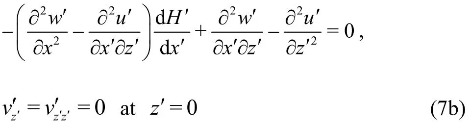
The governing equations for the couple stress fluid, taking into account the rotating frame, will be in the form:


where ρ is the density, μ is the fluid viscosity, η is the couple stress fluid parameter,p′ =p′*-ρΩ2(x′2+y′2) /2 is the modified pressure andp′*is hydrostatic pressure.

Fig.1 Geometry of the problem
Assuming the components of the couple stress tensor are all zero at the wall[1,23], the corresponding non-slip boundary conditions will be:

Consider the following non-dimensional variables and parameters:

whereReis the Reynolds number, δ is the dimensionless wave number, γ (γ>0) is the couple stress fluid parameter indicating the ratio of the channel width (which is constant) to the material characteristic length (since1/2(η/ )μ, has the dimension of length), φ is the amplitude ratio andTrepresents Taylor’s number.
Using the dimensionless variables and parameters given by Eq. (8), together with the stream function ψ(x,z) (such thatu= ψz,w=-δψx), the continuity Eq. (3) is identically satisfied and Eqs.(4)-(6) become:

We define the instantaneous volume flow rate in the fixed frame as follows

whereH′ is function ofX′,t′.
The rate of volume flow in the wave frame is given by

whereh′ is function ofx′ alone. Hence, the two rates of volume flow are related through

The time mean flow over a period τ at a fixed positionxis defined as
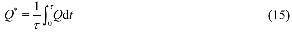
substituting (14) into (15), and integrating, we get

We define the dimensionless time-mean flows θ andFin the fixed and wave frame as:

one finds that (16) may be written as

where

Under lubrication approach (negligible inertiaRe→ 0 and long wavelength δ≪1), the Eqs. (9)-(11) reduce to

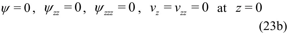
The corresponding boundary conditions will be

2. Solution methodology
Equation (22) shows that the pressurepis not a function ofz. Further,py=0 because the secondary flow is caused by the rotation only. Differentiating Eq. (20) with respect tozand taking into account the above note, one finds that
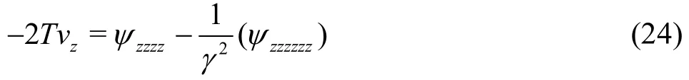
and Eq. (21) will be in the form

To solve Eqs. (24), (25) with the corresponding boundary conditions (23), we are going to use the powerful homotopy perturbation method. The homotopy equation for the given problem is defined as:

whereq∈ [0,1] is the embedded parameter, and L1and L2are the linear operators that are assumed to be L1=∂6/∂z6and L2=∂4/∂z4. We define the initial guess as:

where

Now we describe Substituting the above equation into Eqs. (26),(27) and then taking the terms of order zero, one, and two, we obtain the following models along with the corresponding boundary conditions:
Zeroth-order

with the corresponding boundary conditions

The solution of the zeroth order system can be obtained by using Eqs. (28), (29) and is directly written as

First-order

with the corresponding boundary conditions

The solutions of the above linear ordinary differential equations are found as


Second-order

with the corresponding boundary conditions
The solutions of this order is very large so we omit it from the text. We substitute the values of0ψ,1ψ and2ψ andv0,v1andv2in Eqs. (30), (31),respectively. Now forq→1, we approach the final solutions.
The secondary flow is an indication for the rotating frame in most cases. The physical quantities of interest, such as the dimensionless flow rateF2,due to secondary velocity and the pressure rise Δpare defined, respectively, as:

The shear stress at the wallwτ, after implementing the long wavelength approximation and taking into consideration that the couple stress value vanishes at the wall, will be in the form
3. Quantitative investigation
In this section, theoretical estimates of different physical quantities that are of relevance to the fluid problem have been obtained on the basis of the present study. We investigate novelties brought about by the introduction of Taylor’s numberT, which is due to rotation of channel about thez-axis, and couple stress parameter γ into the model. Particularly, we discuss their effects on the longitudinal velocity distributionu, pressure gradient dp/dx,pressure rise per wavelength Δp, and on the dimensionless flow rate due to secondary velocityF2. The formation of a bolus of fluid which is presented by a snapshot of flow field characteristic streamlines enclosing the pattern is also investigated. For this purpose, the following data that are valid in the physiological range[1,3,7,24]have been used: γ=0.01-3.00,T=0-7, θ= -1 .5-1.5 and φ=0.4-0.6.
3.1 Distribution of velocity
The variations ofTand γ on the longitudinal velocity distributionuhave been portrayed and investigated in this subsection. Figures 2, 3 are constructed to serve this purpose. As shown in Fig.2,the couple stress parameter γ enhances the longitudinal flow velocity and is almost constant within the range 0≤z≤0.2, after which it has a decreasing effect onu. It is obvious that forz≥0.2,udecreases with the variation ofzfor a fixed value of γ. For large values of γ (i.e., move to Newtonian fluid), the longitudinal velocityuincreases in the center region of the fluid layer and decreases near to the wavy walls. Figure 3 elucidates thatuincreases with an increase inTuntil it reaches the center of the channel where the trend is reversed. It is also concluded thatuhas smaller values in the absence of the inertial forces due to rotation till it reaches the center of the channel, where the trend is reversed.Generally, it is obvious thatuattains its maximum value and stays constant over a certain range ofz(0 ≤z≤ 0.2) after which it begins to decrease rapidly.Thus, this considerable increase inu, due to rotation,near the lower wall supports the motion at that zone.Finally, the longitudinal velocity for the rotating fluid is higher than that for non rotating one (T=0). The curves that describe the variation ofufor various values of γ are qualitatively similar to those of Fig.2.
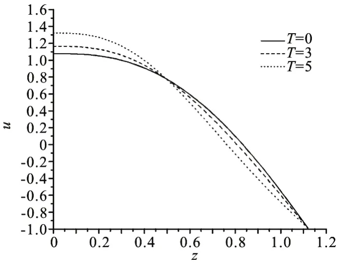
Fig.2 The longitudinal velocity distribution u,across the channel with different values of T at x=0.2, θ=1.5, γ=3.0 and φ=0.4
3.2 Pumping behaviour

Fig.3 The longitudinal velocity distribution u,across the channel with different values of γ at x=0.2,θ=1.5, T=4 and φ=0.4
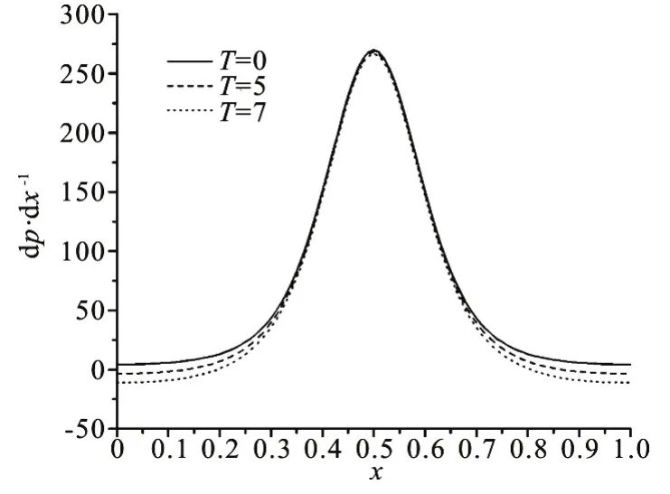
Fig.4 Variation of pressure gradient versus x with different values of T for fixed φ=0.4, θ=-1.5 and γ=2.0
The pumping characteristics can be determined through the variation of time averaged flux with difference in pressure across one wave length. It is known that if the flow is steady in the wave frame, the instantaneous pressure difference between two stations one wave length apart is a constant. Since the pressure gradient is a periodic function of (Z-t), pressure rise per wave length Δpis equal to λ times the time-averaged pressure gradient. The graph is sectored so that the region in which the pressure difference vanishes, Δp=0, is regarded to as the free pumping zone, while the region where Δp>0 (adverse pressure gradient) and θ>0 (positive pumping) is said to be the peristaltic pumping zone where the peristalsis of the walls overcomes the resistance of the pressure and assists the fluid of flow. When Δp>0 and θ<0, the region is known as retrograde or backward pumping where the flux of fluid is opposite to the wave propagation. The situation when Δp<0(favorable pressure gradient) and θ>0 (positive pumping) corresponds to the so-called co-pumping or augmented zone where the pressure difference amplifies the flow. Figures 4, 5 present the variations of dp/dxfor different values ofTand γ where it is noticed that the pressure gradient has a periodic nature. One may observe from Fig.4 that in the range of values of Taylor’s number examined in the present study, the pressure gradient is weakly affected byTin the narrow region of the channel, nevertheless, it has a decreasing effect on the wider region where, it over the ranges of 0 ≤x≤ 0.35 and 0.6≤x≤1,approximately. Generally, the pressure gradient attains its maximum value at the narrow region of the channel from where it decreases rapidly as we go to the wider parts. Figure 5 elucidates that dp/dxis strongly affected by γ which has a decreasing effect on it. It is noticed that the maxima of pressure gradient curve decreases rapidly with an increase in γ. The variations of Δpwith θ for various values ofTand γ are presented in Fig.6. It is seen from the graph that Δpand θ are inversely proportional to each other. Further, Fig.6 shows that upon increasingTand γ, Δpdecreases in the retrograde pumping till a certain value in the peristaltic pumping region after which the pumping rate will increase by increasingTand γ in both, the peristaltic and co-pumping regions. It is observed that the pumping region (Δp>0) decreases with an increase inTfor fixed values of γ. It is also observed that the maximum pressure against which peristalsis works as a positive displacement pump (that is, Δpfor θ=0) decreases for large value ofT(=5). It appears that for the case γ =2, free pumping is independent ofT, but this is not true as seen from the enlargement ofTshown in figure. In contrast, if one keeps increasingT, Δpbecomes negative for most of the positive values of θ. Thus, forT=5, the free pumping is not independent ofT. Hence, for a fluid in a frame rotating with large angular speed, pressure does not rise against the direction of the peristaltic wave. It implies that the pressure assists the flow in such a case.In fact, the rotation of the channel produces a negative secondary component of the velocity which, in turn, is responsible for Coriolis force acting on the fluid in the positivey-direction. This force pulls the fluid outwards and thus, reduces the pressure rise. It is interesting to note that the lines for different values ofTintersect in the region Δp>0. On the other hands,it is noticed from Fig.6 that the pumping region decreases with increasing the values of γ for fixed values ofT. It is also observed that the maximum pressure against which peristalsis works as a positive displacement pump decreases with increasing γ. It appears that free pumping is not independent of γ.Also, if one keeps increasing γ , Δpbecome negative for most of the positive values of θ and the pressure assists the flow. It is interesting to note that the lines for different values of γ intersect in the region Δp<0.

Fig.5 Variation of pressure gradients versus x with different values of γ for fixed φ=0.4, θ=-1.5 and T=0

Fig.6 Variation of pressure rises over the length versus θ with different values of couples tress parameter γ and Taylor’s number T at φ=0.4

Fig.7 The dimensionless flow rates due to secondary velocity F2 for different values of T with φ=0.6, γ=1.0 and θ=-0.2
3.3 Dimensionless flow rate due to secondary velocity
Figures 7, 8 are plotted so as to study the behavior of dimensionless flow rate due to secondary velocity withxfor various values of the concerned parameters. The caseT=0 corresponds to flow rate in the absence of centrifugal forces i.e., the inertial forces due to rotation of channel about thez-axis. It is evident thatF2vanishes when the rotation of channel disappears. For θ=-0.2, it is noticed thatF2is positive in the narrow part of the channel,otherwise, it is negative. It is observed thatThas an increasing effect onF2except over the ranges 0.2≤x≤0.8 and 1.2≤x≤1.8 where the behavior is reversed. Moreover, as the value ofTincreases,F2becomes positive over the whole wavelength of the channel. Figure 8 depicts the influence of couple stress parameter γ onF2for θ=-0.2. It is revealed thatF2is positive over the whole wavelength of the channel for all values of γ. Yet, γ has an increasing effect onF2except for the ranges ofxthat are between 0.2 to 0.8 and 1.2 to 1.8 where the trend reverses.

Fig.8 The dimensionless flow rates due to secondary velocity F2 for different values of γ with φ=0.6, T=2 and θ=-0.2
3.4 Streamlines and trapping
Trapping is an important aspect of peristaltic motion. It occurs when streamlines on the central line are split to enclose a bolus of fluid particles circulating along closed streamlines in the wave frame of reference. Then the fluid particles contained in the bolus move at a mean speed of advance equal to the wave propagation speed, whereas the remaining fluid has a smaller mean speed of advance. Under the purview of the present study, Figs. 9, 10 give an insight into the changes in the patterns of streamlines and trapping that occur due to changes in the values of different parameters governing the flow in the wave frame of reference. Figure 9 illustrates the influence of the rotation of channel on the trapping phenomenon.The caseT=0 corresponds to trapping in the absence of rotation. Here, we observe that the trapped bolus exists about the center streamline. However, the number of closed streamlines circulating the bolus gets raised as we move towards higher values of flow field rotation parameter (increase the values ofT=0,2,5). It is also noticed that the effect ofTis to enhance the area (size) of the trapped bolus with a tendency to move towards the boundary asTincreases. Yet, for small values ofT(=2), there is not much difference in the area trapped bolus compared with that of the absence of rotation case. This phenomenon is useful in understanding the movement of the food bolus in the gastrointestinal tract and the formation of thrombus in blood. Streamlines for various values of the of couple stress parameter γ are depicted in Fig.10. This figure indicates that the occurrence of trapping is strongly influenced by the value of γ. With an increase in γ (move to Newtonian fluid), the bolus is found to appear in a distinct manner and it is observed that the number of closed streamlines circulating the bolus increases.

Fig.9 Streamlines for different values of Taylor’s number T,with fixed values of θ=-1.0, φ=0.4 and γ=2.0
3.5 Distribution of wall shear stress

Fig.10 Streamlines for different values of couple stress parameter γ, respectively, with fixed values of θ=1.0,φ= 0.4 and T=0
It is very interesting to note that for fluids in microcontinuum (couple stress fluids, micropolar fluids,dipolar fluids, etc.), stress tensor is not symmetric. It is known that the stress tensor for a couple stress fluid contains a symmetric and asymmetric parts. And since there are vanishing components of the couple stress tensor at the channel walls, the stress tensor at the wall will have the symmetric part only. Figures 11, 12 display the variation of the symmetric part of the wall shear stress with thex-axis for different values of the couple stress parameter γ and the rotation parameterT. The figures show that the wall shear stress behave just as the wall sinusoidal wave. Further,there exists two peaks in the shear stress distribution,over the rangex=0-2, with a gradual ramp in between. However, the negative peak of the wall shear stress τminis not as large as the maximum wall shear stress, τmax. The transition from τminto τmaxof the wall shear stress takes place in some zone between the minimum and maximum width of the channel.Moreover, an increase in the couple stress parameter γ (i.e., moves towards a Newtonian fluid) and in the rotation parameterTleads to a slight variation in the wall shear stress and this variation is obvious in the bottom area of the wall shear stress wave. However,this variation increases as the rotation parameter increases and is reduced by moving towards a Newtonian fluid (γ take large values ).

Fig.12 Wall shear stress wτ versus x with different values of γ at T=0, φ=0.4 and θ=0.5
4. Concluding remarks
In this study, we investigate the peristaltic flow of a non-Newtonian couple stress fluid in a rotating frame of reference under the long wavelength assumption. The resulting equations are solved, using the powerful HPM, for exact solutions to the longitudinal velocity distribution, pressure gradient, flow rate due to secondary velocity, and pressure rise per wavelength. The main findings can be summarized as follows:
(1) Taylor’s number and the couple stress parameter have an increasing effect onutill half of the channel from where the behavior is reversed.

Fig.11 Wall shear stress wτ versus x with different values of T at γ=2.0 , φ=0.4 and θ=0.2
(2) The pressure gradient, dp/dx, has a periodic nature under the influence of both,Tand γ.
(3) The couple stress parameter strongly affects dp/dxcausing it to decrease, unlikeTwhich weakly affects it.
(4) The pressure rise, Δp, decreases in the retrograde pumping till a certain value in the peristaltic pumping region after which the pumping rate will increase by increasingTand γ in the peristaltic and co-pumping regions.
(5) Free pumping is dependent on high values ofTand on γ in which the pressure does not rise against the direction of the peristaltic wave and hence,assists the flow.
(6) BothTand γ have an increasing effect on the flow rate due to secondary velocity,F2, over certain range ofx.
(7) AsTand γ increase, number of closed streamlines circulating the bolus increases.
(8) The results for the Newtonian incompressible fluid in a rotating frame can be recovered for large values of γ[24].
(9) The shear stress profiles is not significantly disturbed by the numerical value of γ orTin the narrow parts in the channel.
(10) In the absence ofT, our results perfectly match with the results computed on the basis of our study of peristaltic flow of couple stress fluid in the absence of heat transfer in a fixed frame[23].
[1] Stokes V. K. Couple stress fluid [J].Physics of Fluids,1966, 9(9): 1709-1715.
[2] Latham T. W. Fluid motion in a peristaltic pump [D].Master Thesis, Massachusetts, USA: Massachusetts Institute of Technology, 1966.
[3] Noreen S. A., Wahid B. A. Physiological transportation of casson fluid in a plumb duct [J].Communications in Theoretical Physics, 2015, 63(3): 347-352.
[4] Abd elmaboud Y. Thermomicropolar fluid flow in a porous channel with peristalsis [J].Journal of Porous Media, 2011, 14(11): 1033-1045.
[5] Abd elmaboud Y., Mekheimer Kh. S. Non-linear peristaltic transport of a second-order fluid through a porous medium [J].Applied Mathematical Modelling, 2011, 35(6):2695-2710.
[6] Noreen S. A., Wahid B. A. Heat transfer analysis for the peristaltic flow of herschel-bulkley fluid in a nonuniform inclined channel [J].Zeitschrift Für Naturforschung A,2015, 70(1): 23-32.
[7] Noreen S. A. Application of Eyring-Powell fluid model in peristalsis with nano particles [J].Journal of Computational and Theoretical Nanosciences, 2015, 12(1): 94-100.
[8] Ellahi R., Bhatti M. M., Riaz A. et al. The effects of magnetohydrodynamics on peristaltic flow of Jeffrey fluid in a rectangular duct through a porous medium [J].Journal of Porous Media, 2014, 17(2): 143-157.
[9] Hayat T., Asfar A., Khana M. et al. Peristaltic transport of a third order fluid under the effect of a magnetic field [J].Computers and Mathematics with Applications, 2007,53(7): 1074-1087.
[10] Mekheimer Kh. S., Husseny S. Z. A., Abd elmaboud Y.Effects of heat transfer and space porosity on peristaltic flow in a vertical asymmetric channel [J].Numerical Methods for Partial Differential Equations, 2010, 26(4):747-770.
[11] Ellahi R., Bhatti M. M., Vafai K. Effects of heat and mass transfer on peristaltic flow in a non-uniform rectan- gular duct [J].International Journal of Heat and Mass Transfer,2014, 71(4): 706-719.
[12] Mekheimer Kh. S., Abdel maboud Y. Peristaltic flow of a couple stress fluid in an annulus: Application of an endoscope [J].Physica A, 2008, 387(11): 2403-2415.
[13] Hayat T., Wang Y., Siddiqui A. M. et al. Peristaltic transport of a third order fluid in a circular cylindrical tube [J].MathematicalModels and Methods in Applied Sciences,2002, 12(12): 1691-1706.
[14] Hayat T., Wang Y., Siddiqui A. M. et al. Peristaltic transport of an Oldroyd-B fluid in a planar channel [J].Mathematical Problems in Engineering, 2004, 2004(4):347-376.
[15] Nadeem S., Riaz A., Ellahi R. et al. Heat and mass transfer analysis of peristaltic flow of nanofluid in a vertical rectangular duct by using the optimized series solution and genetic algorithm [J].Computational and Theoretical Nanoscience, 2014, 11(4): 1133-1149.
[16] Nadeem S., Riaz A., Ellahi R. Peristaltic flow of viscous fluid in a rectangular duct with compliant walls [J].Computational Mathematics and Modeling, 2014, 25(3):404-415.
[17] Liao S. General boundary element method for non-linear heat transfer problems governed by hyperbolic heat conduction equation [J].Computational Mechanics, 1997,20(5): 397-406.
[18] Liao S. Numerically solving nonlinear problems by the homotopy analysis method [J].Computational Mechanics,1997, 20(6): 530-540.
[19] Ellahi R., Riaz A., Nadeem S. et al. Peristaltic flow of Carreau fluid in a rectangular duct through a porous medium [J].Mathematical Problems in Engineering, 2012,Article ID 329639.
[20] Abd Elmaboud Y., Mekheimer Kh. S., Mohamed M. S.Series solution of a natural convection flow for a Carreau fluid in a vertical channel with peristalsis [J].Journal of Hydrodynamics, 2015, 27(6): 969-979.
[21] Saadatmandi A., Dehghan M., Eftekhari A. Application of He’s homotopy perturbation method for non-linear system of second-order boundary value problems [J].Nonlinear Analysis: Real World Applications, 2009, 10(3):1912-1922.
[22] Mekheimer Kh. S., Abdelmaboud Y., Abdellateef A. I.Particulate suspension flow induced by sinusoidal peristaltic waves through eccentric cylinders: Thread annular[J].International Journal of Biomathematics, 2013, 6(4):1350026.
[23] Abd elmaboud Y., Mekheimer Kh. S., Abdellateef A. I.Thermal properties of couple-stress fluid flow in an asymmetric channel with peristalsis [J].Journal of Heat Transfer, 2013, 135(4): 044502-1.
[24] Ali N., Sajid M., Javed T. et al. Peristalsis in a rotating fluid [J].Scientific Research and Essays, 2012, 7(32):2891-2897.
- 水动力学研究与进展 B辑的其它文章
- Numerical analyses of ventilated cavitation over a 2-D NACA0015 hydrofoil using two turbulence modeling methods *
- Analytical approach to entropy generation and heat transfer in CNT-nanofluid dynamics through a ciliated porous medium *
- 2-D eddy resolving simulations of flow past a circular array of cylindrical plant stems *
- Revisit submergence of ice blocks in front of ice cover-an experimental study *
- Energy dissipation of slot-type flip buckets *
- Some notes on numerical simulation and error analyses of the attached turbulent cavitating flow by LES *