
A Diagonalized Legendre Rational Spectral Method for Problems on the Whole Line
2018-08-06 06:10XuhongYuYungeZhaoandZhongqingWang
Journal of Mathematical Study 2018年2期
Xuhong Yu,Yunge Zhao and Zhongqing Wang
School of Science,University of Shanghai for Science and Technology,Shanghai,200093,P.R.China.
Abstract.A diagonalized Legendre rational spectral method for solving second and fourth order differential equations are proposed.Some Fourier-like Sobolev orthogonal basis functions are constructed which lead to the diagonalization of discrete systems.Accordingly,both the exact solutions and the approximate solutions can be represented as in finite and truncated Fourier series.Numerical results demonstrate the effectiveness of this approach.
AMS subject classifications:65N35,41A20,33C45,35J25,35J40,35K05
Key words:Legendre rational spectral method,Sobolev orthogonal functions,elliptic boundary value problems,heat equation,numerical results.
1 Introduction
Many science and engineering problems are set in unbounded domains,such as fl uid flows in an in finite strip,nonlinear wave equations in quantum mechanics and so on.How to accurately and efficiently solve such problems is a very important and dif ficult subject,since the unboundedness causes considerable theoretical and practical challenges.There are several ways for their numerical simulations.Usually we restrict calculations to some bounded subdomains and impose certain artificial boundary conditions.It is easy to be performed,but it lowers the accuracy sometimes.The second way is to use spectral method associated with some orthogonal systems on the unbounded domains,such as the Laguerre and Hermite spectral method[1,2,5,6,8–10,13,16–19].However,since the Laguerre/Hermite Gauss points are too concentrated near zero,the approximation results are usually not ideal,especially where the points are far away from zero.The third method is to change original problems by variable transformations to certain singular problems on finite intervals,and then use Jacobi approximation to resolve the resulting problems[7].The fourth effective method is to use algebraically mapped Legendre,Chebyshev or Jacobi functions to approximate the differential equations,i.e.,the so-called Legendre,ChebyshevorJacobi rational spectralmethod[3,4,11,12,21,22].Compared with the first three methods,we prefer the last way,since the distribution of the Gauss points is more reasonable than that of Laguerre and Hermite Gauss points.
As is well known,the utilization of Legendre rational functions usually leads to a highly sparse algebraic system(a nine-diagonal matrix for second order problems and a seventeen-diagonalmatrix for fourth order problems),the condition numbers increase as O(N2)for the second order problem andO(N4)for the fourth order problem.However,in many cases,researchers still want a set of Fourier-like basis functions for a diagonalized algebraic system[14,15,20].Motivated by[14,15,20],the main purpose of this paper is to construct the Fourier-like Sobolev orthogonalbasis functions and proposethe diagonalized Legendre rational spectral method for second and fourth problems on the whole line.
The main advantages of the suggested algorithm include:(i)The exact solutions and the approximate solutions can be represented as in finite and truncated Fourier series,respectively;(ii)The condition numbers for the resulting algebraic systems are equal to 1;(iii)The computational cost is much less than that of the classical Legendre rational spectral method.
This paper is organized as follows.In Section 2,we introduce the modified Legendre rational functions and its basic properties.In Section 3,we construct the Sobolev orthogonal Legendre rational functions corresponding to the second order elliptic equation,the fourth order elliptic equation and the nonlinear heat equation,and propose the diagonalized Legendre rational spectral methods.Some numerical results are presented in Section 4 to demonstrate the effectiveness and accuracy.
2 Modified legendre rational functions
We first recall the Legendre polynomials.Let I={y|−1<y<1}and Lk(y)be the Legendre polynomial of degree k,which is the eigenfunction of the singular Sturm-Liouville problem:

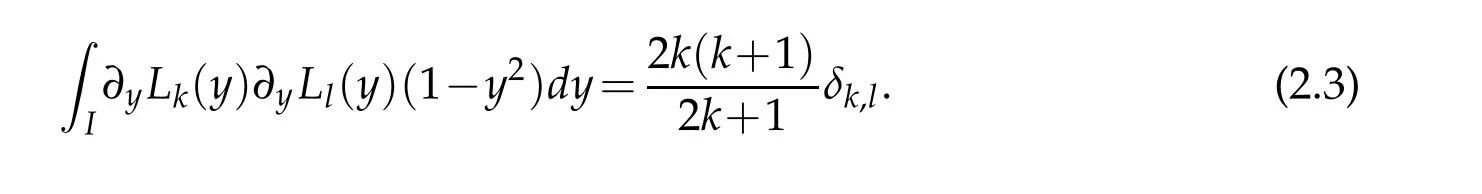
The set of all Legendre polynomials forms a complete L2(I)-orthogonal system,namely,

where δk,lis the Kronecker function.By virtue of(2.1)and(2.2),we have
Moreover,for any k≥1,the following recurrence relations are satisfied with L0(y)=1 and L1(y)=y,
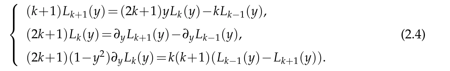
Besides,Lk(±1)=(±1)kand ∂yLk(±1)=(±1)k+1k(k+1).
We next recall the modifiedLegendrerational functions.Let Λ={x|−∞<x<∞}and(u,v)be the inner product of the space L2(Λ).The modified Legendre rational function of degree k is defined by(cf.[21])

Forconvenience,let Rk(x)≡0 forany integerk<0.Due to(2.4),themodified Legendrerational functions satisfy the following recurrence relations with

The set of{Rk(x)}k≥0forms a complete L2(Λ)-orthogonal system,

Moreover,by(2.3)we know that the functions∂x((x2+1)34Rk(x))are mutually orthogonal with respect to the weight function χ1(x)=(x2+1)12,

Lemma 2.1.For any k≥0,we have

and
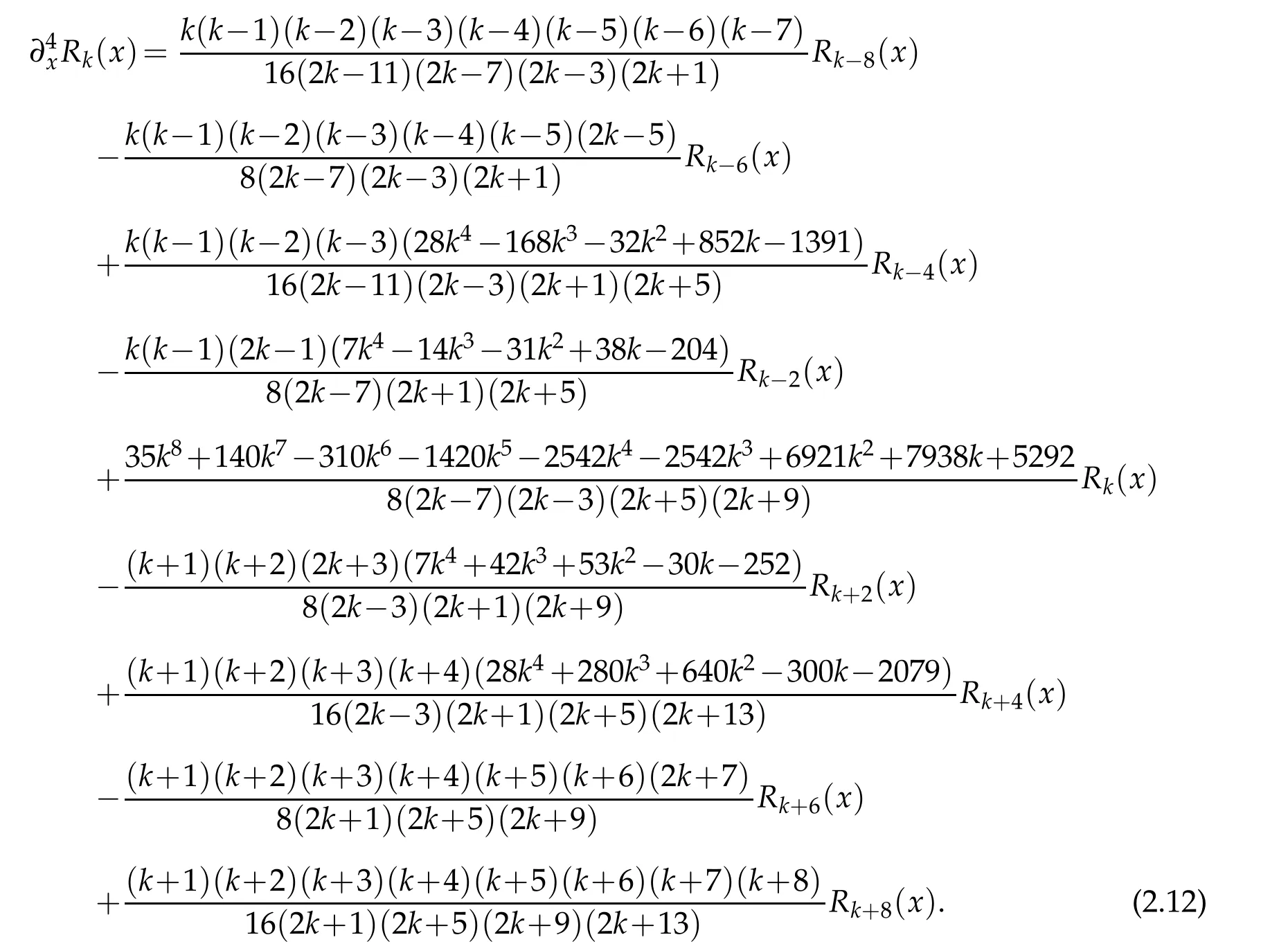
Proof.By(2.8),(2.6)and(2.7),we derive that

Next,denote by A=(ak,l)0≤k,l≤Nthe matrix with the element ak,l=(∂xRl,∂xRk).By using(2.13)and(2.10),we can deduce readily the nonzero elements of matrix A as follows,
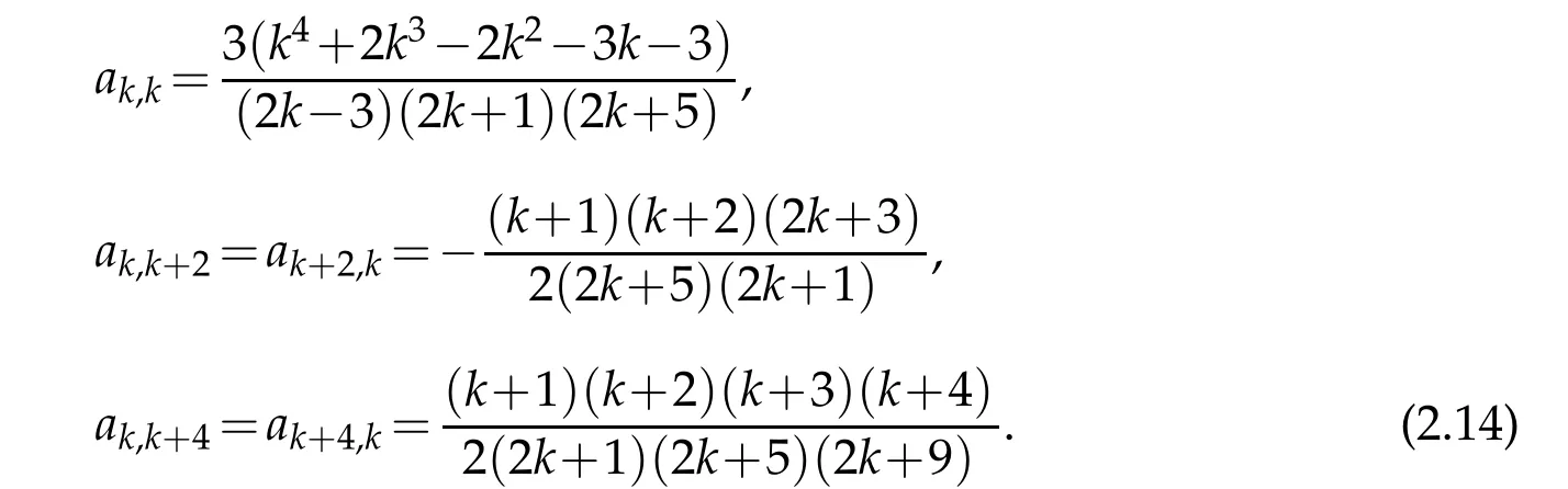
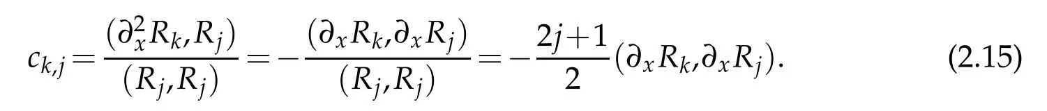
This,along with(2.14),leads to the result(2.11).In the same manner,we derive the result(2.12).
3 Diagonalized Legendre rational spectral methods
In this section,we propose a diagonalized Legendre rational spectral method for solving various differential equations.
3.1 Second-order problems
Consider the second order elliptic boundary value problem:
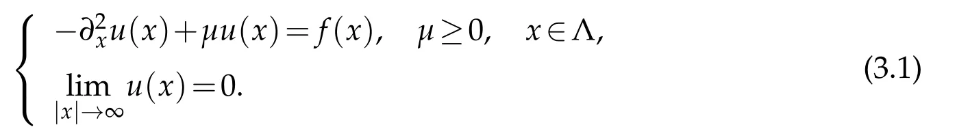
A weak formulation of(3.1)is to find u∈H1(Λ)such that

Clearly,if f∈(H1(Λ))′,then by Lax-Milgram lemma,(3.2)admits a unique solution.
Next,let N be any positive integer,andRN(Λ)=span{R0(x),R1(x),···,RN(x)}.The Legendre rational spectral scheme for(3.2)is to find uN∈RN(Λ)such that

To propose a diagonalized approximation scheme for(3.3),we need to construct new basis functions{ϕk}0≤k≤N,which are mutually orthogonal with respect to the Sobolev inner produce Aµ(·,·).
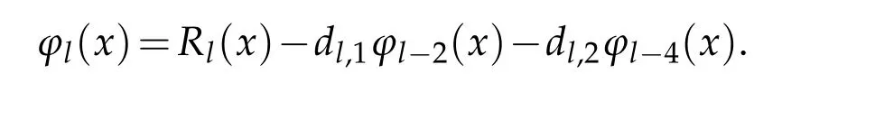
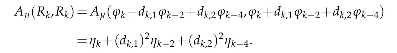
Lemma 3.1.Let ϕk∈ Rk(Λ)be the Sobolev orthogonal Legendre rational function such that ϕk−Rk∈Rk−1(Λ)and

Then we have

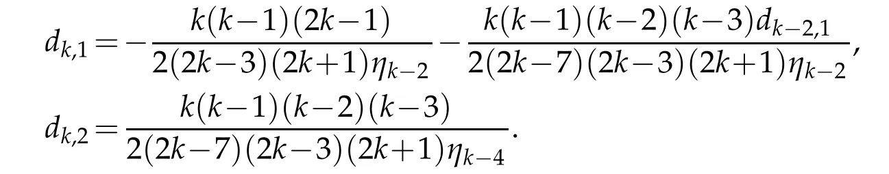
where ϕk(x)≡0(k<0),ηk=0(k<0),dk,1=0(k<2),dk,2=0(k<4),and

Proof.We first use mathematical induction to verify the result(3.5).According to the orthogonality assumption(3.4),we have

Due to the orthogonality(2.9),we know

Therefore,with the help of(2.11),we obtain that
1.2.3 血压测量:采取经校正的台式血压计,在受试者静坐5~10分钟后采取右臂测量2次,每次间隔至少1分钟,取3次均值为其血压值。

This means ϕ1(x)=R1(x).Similarly,

which means ϕ2(x)=R2(x)−d2,1ϕ0(x)with the constantIn the same manner,we can verify the results of(3.5)for k=3,4,with the constantsandas in(3.6).
Next,assume that for any 0≤l≤k−1 and k≥5,
We shall prove that for k≥5,

In fact,by(3.2),(3.8),(2.11)and the induction assumption,we derive that for k>l≥0 and k≥5,

Hence,by(3.7)we verify the result(3.5)with
It remains to confirm the constant ηk.Clearly,by(2.9)and(2.11)we get

On the other hand,by(3.5)we have

This ends the proof.
Obviously,RN(Λ)={ϕk(x):0≤k≤N}.Thus the variational forms(3.2)and(3.3)together with the orthogonality of{ϕk(x)}lead to the following main theorem in this subsection.
Theorem 3.1.Let u(x)and uN(x)be the solution of(3.1)and(3.3),respectively.Then both u(x)and uN(x)have the explicit representations in{ϕk(x)},

3.2 Fourth-order problems
Consider the fourth order elliptic boundary value problem:

A weak formulation of(3.10)is to find u∈H2(Λ)such that

Clearly,if f∈(H2(Λ))′,then by Lax-Milgram lemma,(3.11)admits a unique solution.
The Legendre rational spectral scheme for(3.11)is to find uN∈RN(Λ)such that

Toproposeadiagonalized approximation schemefor(3.12),weneedto constructnew basis functions{ψk}0≤k≤N,which are mutually orthogonal with respect to the Sobolev inner produce Bα,β(·,·).
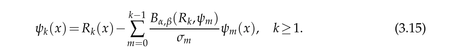
Lemma 3.2.Let ψk∈ Rk(Λ)be the Sobolev orthogonal Legendre rational functions such that ψk−Rk∈Rk−1(Λ)and

Then the following recurrence relation holds:

where ψk(x)≡0(k<0),σk=0(k<0),ak=0(k<2),bk=0(k<4),ck=0(k<6),dk=0(k<8),and


Proof.According to the orthogonality assumption(3.13),we have
We first use mathematical induction to verify(3.14).By(2.9)we have(Rk,ψm)=0,∀ m<k.Therefore,by(2.11)and(2.12)we obtain

Thus,ψ1(x)=R1(x).Similarly,

which means ψ2(x)=R2(x)−a2ψ0(x)with the constantIn the same manner,we can verify the results of(3.14)for k≤8.
Next,assume that for any 0≤l≤k−1 and k≥9,

We shall prove that for k≥9,

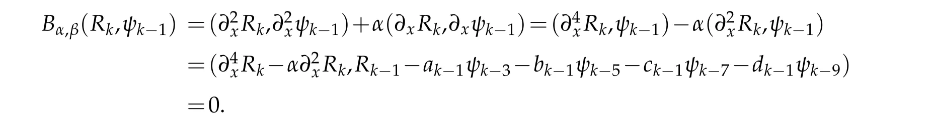
In fact,by(2.9)and(3.11),we deduce that for any k>m≥0,

From(2.11),(2.12)and(2.9),we know thatfor 0≤m≤k−9 and 0≤n≤k−5.Therefore,by(3.15)we get

Next,by(2.11),(2.12),(2.9),(3.13)and the induction assumption,we know that for k≥9,
On the other hand,

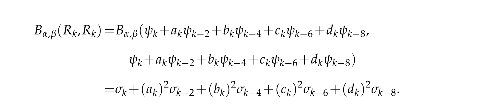
It remains to confirm the coefficients ak,bk,ck,dkand σk.Actually,by using(2.11),(2.12)and(2.9),we obtain that for k>m≥0 and k≥9,

On the other hand,

Taking m=k−2,k−4,k−6,k−8 in(3.17)and(3.18)respectively,we derive the results(ii)-(v)in Lemma 3.2.
We next confirm the constant σk.By using(2.11),(2.12),(2.9)and(3.13),we know that for k≥9,

and
This gives the result(i)of Lemma 3.2.
Theorem 3.2.Let u(x)and uN(x)be the solution of(3.10)and(3.12),respectively.Then both u(x)and uN(x)have the explicit representations in{ψk(x)},

3.3 The nonlinear heat equation
Consider the following nonlinear heat equation,
whereµ>0 and f(x,t)is a given function.
We shall propose an efficient spectral- finite difference scheme based on diagonalized Legendre rational spectral method in space and the finite difference method in time.
Denote by τ the time step size,M=,and u(k)(x)=u(x,kτ),k=0,1,2,···,M.Then,a standard centered difference scheme in time is given by
A weak formulation of(3.20)is to find u(k+1)(x)∈H1(Λ)such that

where

The Legendre rational spectral scheme for(3.21)is to findsuch that

where

To propose a diagonalized Legendre rational spectral scheme for(3.22),we need to constructnewbasis functions{Ψk(x)}0≤k≤N,whichare mutually orthogonalwithrespect to the Sobolev inner produce Aτ,µ(·,·).
Lemma 3.3.Let Ψk∈ Rk(Λ)be the Sobolev orthogonal Legendre rational functions such that Ψk−Rk∈Rk−1(Λ)and

Then we have

where Ψk(x)≡0(k<0),γk=0(k<0),dk,1=0(k<2),dk,2=0(k<4),and

Proof.The proof is in the same way as Lemma 3.1.We neglect the details.
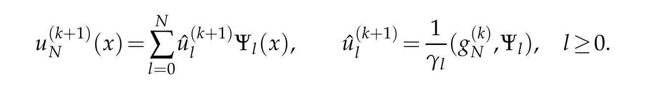
Theorem 3.3.Letbe the solution of(3.22).Then we have
Remark 3.1.This is an implicit scheme.In actual computation,an iterative process should be employed to evaluate the expansion coefficients.
4 Numerical results
Inthis section,weexamine theeffectivenessand theaccuracy ofthediagonalized Legendre rational spectralmethod for solving elliptic equations and nonlinear heat equation.
We first examine the secondorderproblem(3.1)withµ=1,and considerthe following two cases of the smooth solutions with different decay properties.
• u(x)=e−x2sin(kx),which is exponential decay with oscillation.In Figure 1,we plot the log10of the discrete L2-and H1-errors vs.N with k=2.The two near straight lines indicate a geometric convergence rate.
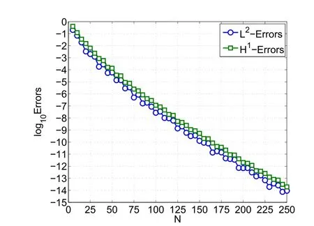
Figure 1:Errors of scheme(3.3)with exponential decay function.

Figure 2:Errors of scheme(3.3)with algebraic decay function.
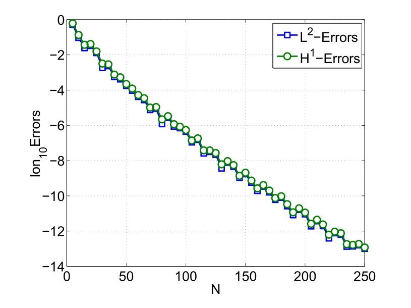
Figure 3:Errors of scheme(3.12)with exponential decay function.

Figure 4:Errors of scheme(3.12)with algebraic decay function.
We next examine the fourth order problem(3.10)with α= β=1,and consider the following two cases of the smooth solutions with different decay properties.
•u(x)=e−x2sin(kx),which is exponential decay with oscillation.In Figure 3,we plot the log10of the discrete L2-and H1-errors vs.N with k=2.Again,a geometric convergence rate is observed.
We finally consider the nonlinear heat equation(3.19)withµ=1,and consider the following two cases of the smooth solutions with different decay properties.
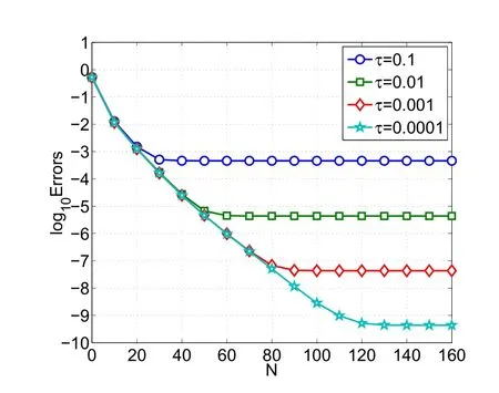
Figure 5:L2-errors of scheme(3.22)with exponential decay function.

Figure 6:H1-errors of scheme(3.22)with exponential decay function.

Figure 7:Stability of scheme(3.22)with exponential decay function.
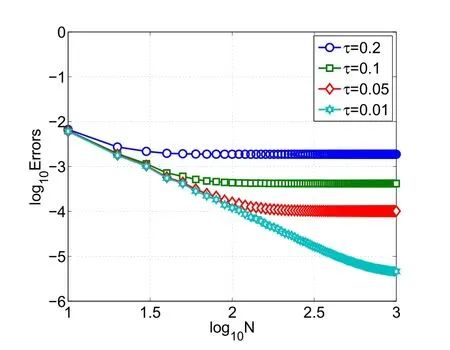
Figure 8:L2-errors of scheme(3.22)with algebraic decay function.
• u(x,t)=e−x2sin(k1x+k2t),which is exponential decay with oscillation.In Figures 5 and 6,we plot the log10of the discrete L2-and H1-errors vs.N with τ=0.1,0,01,0.001,0.0001 and k1=2,k2=1,respectively.Clearly,a geometric convergence rate is observed.They also indicate that the smaller the time step size τ,the smaller the numerical errors would be.In Figure 7,we plot the values of L2-errors for 0≤t≤100 with τ =0.01.It demonstrates the stability of long-time calculation of scheme(3.21).
To demonstrate the essential superiority of the diagonalized Legendre rational spectral method to the classic Legendre rational and Hermite spectral methods,we also ex-amine the issues on the condition numbers for the resulting algebraic systems and the computational cost.

Table 1:Condition numbers of the classical Legendre rational spectral method
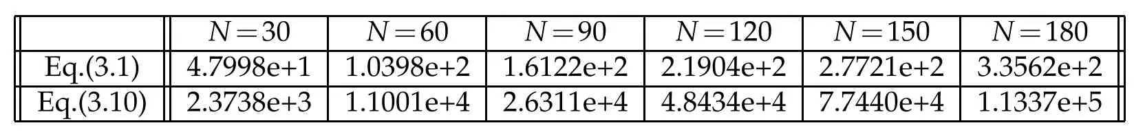
Table 2:Condition numbers of Hermite spectral method

Table 3:Diagonalized Legendre rational spectral method for(3.10).

Table 4:Classical Legendre rational spectral method for(3.10).
The basis functions in the diagonalized Legendre rational spectral method are chosenandwhich are Sobolev orthogonal.Accordingly,the condition numbers are equal to 1.
For the classical Legendre rational and Hermite spectral methods,the basis functions are chosen asThe corresponding stiff matrices have off-diagonal entries.In Tables 1 and 2 below,we list the condition numbers of the classical Legendre rational spectral method and Hermite spectral method for(3.1)and(3.10).Note that the condition numbers in Table 1 increase asO(N2)for the second order problem(3.1)andO(N4)for the fourth order problem(3.10)by the classical Legendre rational spectral method with α=β=µ=1.Moreover,the condition numbers in Table 2 increase asO(N)for the second order problem(3.1)andO(N2)for the fourth order problem(3.10)by the Hermite spectral method with α=β=µ=1.
For comparison of the computational cost between the diagonalized Legedre rational spectral method and the classical Legedre rational spectral method,we consider the problem(3.10)with α=β=1.In Tables 3 and 4,we list the L2-errors and the corresponding computational cost.It can be observed that our diagonalized spectral method costs much less CPU time.
Acknowledgments
This work was supported in part by NSF of China No.11571238 and No.11601332 and the Hujiang Foundation of China No.B14005.
猜你喜欢
家庭医药(2021年16期)2021-12-02
家庭医药·快乐养生(2021年8期)2021-08-30
中学生数理化·八年级物理人教版(2021年4期)2021-07-22
工业设计(2019年9期)2019-11-04
党的生活(黑龙江)(2019年5期)2019-06-11
青年文学家(2017年28期)2017-11-28
中国棉花(2017年10期)2017-11-04
海峡姐妹(2017年7期)2017-07-31
中国新闻周刊(2017年19期)2017-06-01
少林与太极(2014年9期)2014-10-15
 Journal of Mathematical Study2018年2期
- Journal of Mathematical Study的其它文章
- Ill-posedness of Inverse Diffusion Problems by Jacobi’s Theta Transform
- Highly Efficient and Accurate Spectral Approximation of the Angular Mathieu Equation for any Parameter Values q
- POD Applied to Numerical Study of Unsteady Flow Inside Lid-driven Cavity
- Generalized Hermite Spectral Method for Nonlinear Fokker-Planck Equations on the Whole Line
- Chebyshev Spectral Method for Volterra Integral Equation with Multiple Delays