A CORRECTOR-PREDICTOR ARC SEARCH INTERIOR-POINT ALGORITHM FOR SYMMETRIC OPTIMIZATION∗

M.PIRHAJIM.ZANGIABADIH.MANSOURI

Department of Applied Mathematics,Faculty of Mathematical Sciences,Shahrekord University,Shahrekord,Iran

E-mail:mojtabapirhaji@yahoo.com;Zangiabadi-m@sci.sku.ac.ir;mansouri@sci.sku.ac.ir

Abstract In this paper,a corrector-predictor interior-point algorithm is proposed for symmetric optimization.The algorithm approximates the central path by an ellipse,follows the ellipsoidal approximation of the central-path step by step and generates a sequence of iterates in a wide neighborhood of the central-path.Using the machinery of Euclidean Jordan algebra and the commutative class of search directions,the convergence analysis of the algorithm is shown and it is proved that the algorithm has the complexity bound O(√rL)for the well-known Nesterov-Todd search direction and O(rL)for the xs and sx search directions.

Key words symmetric optimization;ellipsoidal approximation;wide neighborhood;interiorpoint methods;polynomial complexity

1 Introduction

Symmetric optimization(SO)problem is a special class of convex optimization problems in which a linear function is minimized over the intersection of an affine subspace and a closed convex cone.The SO problem includes the well-known and well-studied optimization problems such as linear optimization(LO)problems,semidefinite optimization(SDO)problems and second order cone optimization(SOCO)problems.Thus,the considerable attention has been devoted by the researchers to solve this class of mathematical programming.

The first attempts for solving SO problems,using interior-point methods(IPMs),was laid by Nesterov and Nemirovskii[1].Using the Euclidean Jordan algebras(EJAs),Faybusovich[2]generalized IPMs for SDO problems to SO problems.Monteiro and Zhang[3],based on the so-called Nesterov-Todd(NT),XS and SX search directions,designed the primal-dual IPMs for SDO problems.After that,Schmieta and Alizadeh[4]proved the convergence analysis and the polynomial complexity bound of short-,semi-long-and long-step IPMs for SO problems using the NT,xs and sx search directions.

Among various types of primal-dual IPMs,predictor-corrector interior-point algorithms are the most applicable and efficient methods theoretically and computationally.The first predictorcorrector interior-point algorithm was proposed by Mehrotra[5].Salahi and Mahdavi-Amiri[6]proposed a new variant of Mehrotra-type algorithm for LO and proved that their algorithm will terminate after at most O?nlogε−1?iterations using a strictly feasible starting point.Liu et al.[7]generalized the proposed algorithm by Salahi and Mahdavi-Amiri[6]for LO to SO problems and proved,using the NT-search direction,the complexity bound O?rlogε−1?for their algorithm,where r is the rank of the associated EJA.

The Mizuno-Todd-Ye(MTY)predictor-corrector interior-point algorithm[8]has done well in both theoretical and computational aspects.Ye et al.[9]proved the superlinear convergence of MTY algorithm.A wide-neighborhood MTY-type predictor-corrector interior-point algorithm suggested by Yang et al.[10]for SO problems.They proved the convergence analysis of their algorithm and obtained the complexity boundsand for the so-called NT and xs and sx search directions.

The most of above mentioned interior-point algorithms follow the central path to reach an ε-optimal solution of the underlying problems in a sufficiently small neighborhood of the central-path.However,following the central path is the main difficulty of IPMs.Therefore,it is worth to investigate the analysis of some interior-point algorithms that approximate the central-path by some arcs.The idea of approximating the central-path by an ellipse was first introduced by Yang[11,12]for convex quadratic optimization(CQO)and LO problems.

Searching along the ellipse is more efficient than searching along any straight line due to generating a larger step size.Indeed,Yang[11]showed that the arc-search algorithm has the best polynomial bound and it may be very efficient in practical computation.Moreover,this result was extended to prove a similar result for CQO problems and the numerical test result was very promising[12].

Yang[13]proposed an arc search infeasible interior-point algorithm for LO and established that under some conditions the computational performance of his algorithm is more efficient than the well-known Mehrotra predictor-corrector(MPC)interior-point algorithm[5].Yang et al.[14,15]proposed two arc search infeasible interior-point algorithms for LO and SO problems,established their convergence analysis and proved that these algorithms respectively will terminate after at mostiterations anditerations using the NT-search direction.

An O(nL)-predictor-corrector arc search interior point algorithm has been proposed by Yang and Yamashita[16]for LO.Using an ℓ2-neighborhood and the arc search strategy,Pirhaji et al.[17]suggested an infeasible interior-point algorithm for linear complementarity problems.

In this paper,motivated by these works,we propose a corrector-predictorarc-searchinteriorpoint algorithm for SO problems.The algorithm uses a wide neighborhood of the central path and involves two kind of steps:a corrector step and a predictor step.In the corrector step,using the corrector directions,the algorithm follows the ellipsoidal approximation of the central path for moving to a smaller neighborhood of the central path and improving the centrality and optimality.Then,in order to further improvement of optimality,the algorithm takes a predictor step by using the affine search directions and moves back toward the slightly larger neighborhood of the central path from the corrector point.

We prove the convergence analysis of the algorithm and show that the proposed algorithm will terminate after at mostiterations using the NT search direction while it needs to perform at most O(rL)iterations by the xs and sx search directions.These iteration bounds match the currently best-known ones for solving SO problems.

The paper is organized as follows.In Section 2,we provide some basic concepts on Euclidean Jordan algebras which are required in our analysis.Section 3 provides some preliminaries on SO problems,the central path and its ellipsoidal approximation.An algorithmic framework of arc search corrector-predictor interior-point algorithm is presented in Section 4.Some technical lemmas which play an important role in proof of convergence analysis of the algorithm will be presented in Section 5.The convergence analysis and the polynomial complexity of the proposed algorithm will be investigated in Section 6.Finally,the paper ends with some concluding remarks in Section 7.

2 Euclidean Jordan Algebras

In this section,we briefly review the necessary background of EJAs and symmetric cones.The background material and the notations in this section are taken from Faraut and Koranyi[18].A Jordan algebra J is a finite dimensional vector space over the field of real or complex numbers endowed with a bilinear map◦:J×J→J satisfying the following properties for all x,y∈J:

(i)x◦y=y◦x,

(ii)x◦(x2◦y)=x2◦(x◦y),

where x2:=x◦ x.Moreover,(J,◦)is called a Euclidean Jordan algebra(EJA)if there exists an inner product denoted by h·,·i such that hx ◦ y,zi=hx,y ◦ zi for all x,y,z ∈ J.

A Jordan algebra has an identity element,if there exists a unique element e∈J such that x◦e=e◦x=x for all x∈J.The set K:=K(J)={x2:x∈J}is called the cone of squares of EJA(J,◦,h·,·i)and int(K)denotes the interior of K.A cone is symmetric if and only if it is the cone of squares of a EJA.

An element c∈J is said to be idempotent if c2=c.An idempotent c is primitive if it is nonzero and can not be expressed by sum of two other nonzero idempotents.A set of idempotents{c1,c2,···,ck}is called a Jordan frame if ci◦cj=0 for any i 6=j,and

For any x ∈ J,let l be the smallest positive integer such that{e,x,x2,···,xl}is linearly dependent,l is called the degree of x and is denoted by deg(x).The rank of J,denoted by rank(J),is defined as the maximum of deg(x)over all x∈J.

Due to Theorem III.1.2 in[18],for any x∈J there exist the unique and distinct real numbers λ1(x),λ2(x),···,λn(x)and Jordan frame{c1,c2,···,cn}such thatEvery λi(x)is called an eigenvalue of x.We denote λmin(x)(λmax(x))as the minimal(maximal)eigenvalue of x.For any x∈J,we define the merit projectionwherefor i=1,2,···,k.

Since“◦”is a bilinear map,for every x ∈ J,a linear operator L(x)can be defined such that L(x)y=x◦y for all y∈J.In particular,L(x)e=x and L(x)x=x2.For each x∈J,we define

where L(x)2:=L(x)L(x).The map Qxis called the quadratic representation of x.The quadratic representation is an essential concept in theory of Jordan algebras and plays an important role in convergence analysis of IPMs in SO.

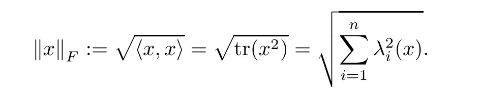
For any x,y∈J,x and y are said to be operator commute if L(x)and L(y)commute,i.e.,L(x)L(y)=L(y)L(x).We define the inner product of x,y∈J as hx,yi=tr(x◦y).The norm induced by this inner product is named as the Frobenius norm,which is given by

3 Preliminaries

Let J be an EJA of dimension n and rank r,and K be its associated cone of squares.Let the standard primal-dual pair of SO problems

and

where c∈J,b∈Rm,A is a linear operator that maps J into Rmand A∗is its adjoint operator such that hx,A∗yi=hAx,yi for all x∈ J.

Throughout this paper,we assume rank(A)=m and the SO problem satisfies the interiorpoint condition(IPC).That is,F06=∅,where

Under the IPC, finding an optimal solution of(3.1)and(3.2)is equivalent to solving the following system:

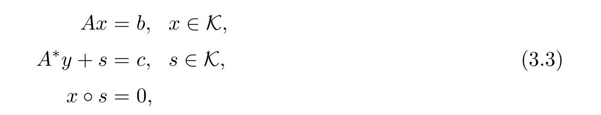
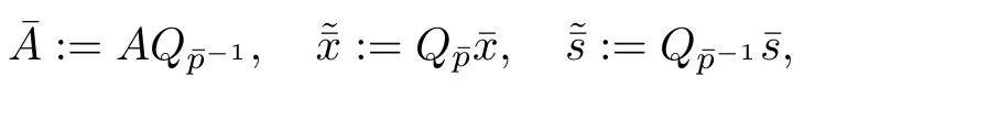
where the third equation is called the complementarity condition.Replacing x◦s=0 by the perturbed complementarity condition x◦s=µe withusing Lemma 28 in[4]for a scaling point p∈C(x,s),where

and defining

system(3.3)can be rewritten as follows:

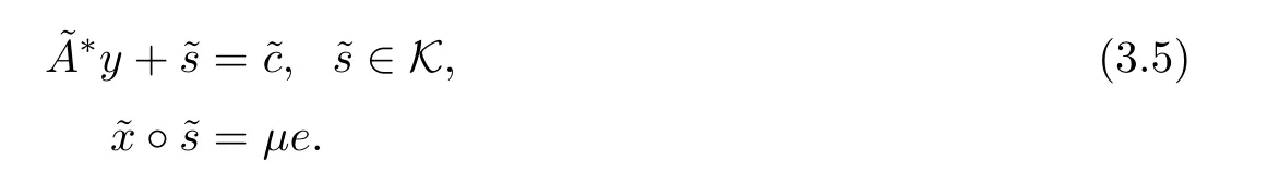
This system,for eachµ>0,has the unique solutionThe set of these solutions constructs a parameterized curve in R2n+m,namely,the feasible central path.It is well-known ifµ → 0,then the limit of the central path exists and yields an ε-optimal solution of SO(see Faybusovich[2]).

Different choices of the scaling point p led to the different search directions.For instance,the choices p:=and p:=,respectively led to the well-known xs and sx search directions while for the choice of

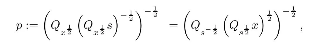
we get the NT search direction.

An important ingredient of this paper is to use the following neighborhood of the central path:

Although,the most of IPMs follow the central path approximately to get close enough to an ε-optimal solution of the problem but following the central path is the main difficulty of interior-point algorithms in practical applications.To this end,motivated by Yang[11,12],we estimate the central path of the SO problem by the ellipse ξ(θ) ∈ R2n+mdefined by Carmo[19]:

Mathematically,an ellipse can be determined by a point on the ellipse and the first and second derivatives at that point.On the other hand,the main idea of arc search IPMs is to estimate the central path of the underling problem by an ellipse.Therefore,to estimate the central path of SO problem by the ellipse ξ(θ),assumingwe proceed to determine the vectorsthe anglesuch that the first and second derivativesofhavethe form as if they wereon the central path.

However,usingthe approach of Yang[11,12],we defineas the first and second derivatives of(x,y,s)to satisfy

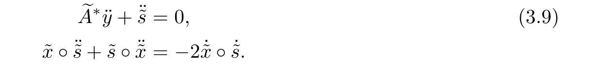
Lemma 3.1(Lemma 3.1 in[11]) Let ξ(θ)be the defined ellipse in(3.7)which passes a pointMoreover,assume that the first and second derivativessatisfy(3.8)and(3.9).Then,after searching along the ellipse ξ(θ),the new generated pointis given by

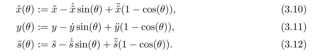
Due to the above lemma,the ellipsoidal approximation of the central path is defined as follows

4 Arc Search Corrector-Predictor Algorithm

In this section,we explain our algorithm for SO.Let the initial starting pointwith the duality gapis available.The algorithm first performs a corrector step to obtain a new iterate that improves both optimality and centrality.

Motivating by[15,22],we modify system(3.8)and define the first and second derivatives at(x,y,s)in the corrector step to satisfy

Now,in order to further improvement of the optimality,starting from the corrector pointchoosing the scaling point p related to( x, y, s)and defining

the algorithm computes the predictor directions

Finally,the algorithm calculates the maximum step size sin()and obtains the predictor point∈NF(τ,β)withThis procedure will be repeated until an ε-optimal solution of the problem is found.

The generic framework of our algorithm is presented bellow.

Algorithm 1(Corrector-predictor arc search interior-point algorithm for SO)

• Input parameters An accuracy parameter ε>0,a neighborhood parameter β ∈ (0,],a centering parameter τ∈(0,],an initial point(x0,y0,s0)∈NF(τ,β)withµ0=tr?◦s0?.

• Step 0 Set k=0,1,2,···.

•Step 1Ifµk≤εµ0,stop.Otherwise go to the next step.

•Step 2(Corrector-step)Compute the corrector directionsrespectively by systems(4.1)and(4.2)and obtain the largest step size sin(ˆθk)such that

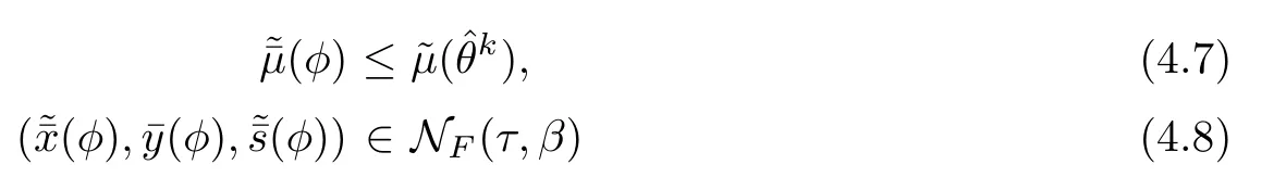
for any step size sin(φ)∈[0,sin(k)].•Step 5Computeand go to Step 1.

5 Technical Lemmas

In this section,some required technical lemmas in order to demonstrate the convergence analysis of Algorithm 1 are presented.

Lemma 5.1(Lemma 6.1 in[20])Letthen

Lemma 5.2(Lemma 33 in[4]) Let u,v∈J and G be a positive definite matrix which is symmetric with respect to the scalar product.Then

Lemma 5.3(Lemma 2.15 in[21]) If x◦s∈intK,then det(x)6=0.

Lemma 5.4(Lemma 5.7 in[22])Let x,s∈J.Then

Lemma 5.5(Lemma 30 in[4])Let x,s∈intK,and w:=s.Then

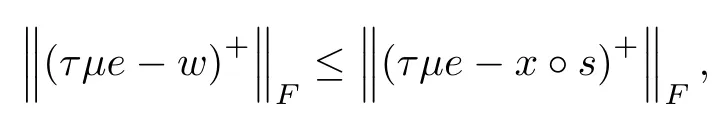
where τ∈ (0,1)and µ >0.If x and s operator commute,then equality holds.

Lemma 5.6(Lemma 2.9 in[23]) Let x,s∈J,then

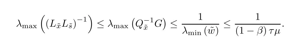
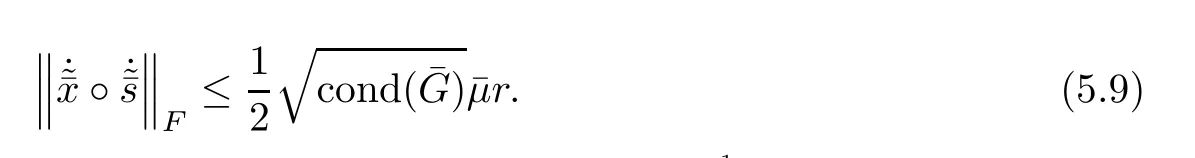
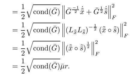
Lemma 5.7(Lemma 5.3 in[22])Let(x,s)∈NF(τ,β)andThen

ProofMultiplying the last equation of system(4.1)bytaking squared norm on both sides and using the fact trand Lemmas 5.6,5.2 and 5.7,we derive

The proof is completed.

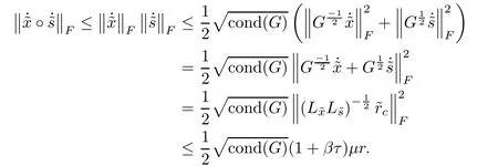
On the other hand,multiplying the last equation of system(4.2)bytaking squared norm on both sides and using Lemmas 5.1 and 5.8,it radially follows

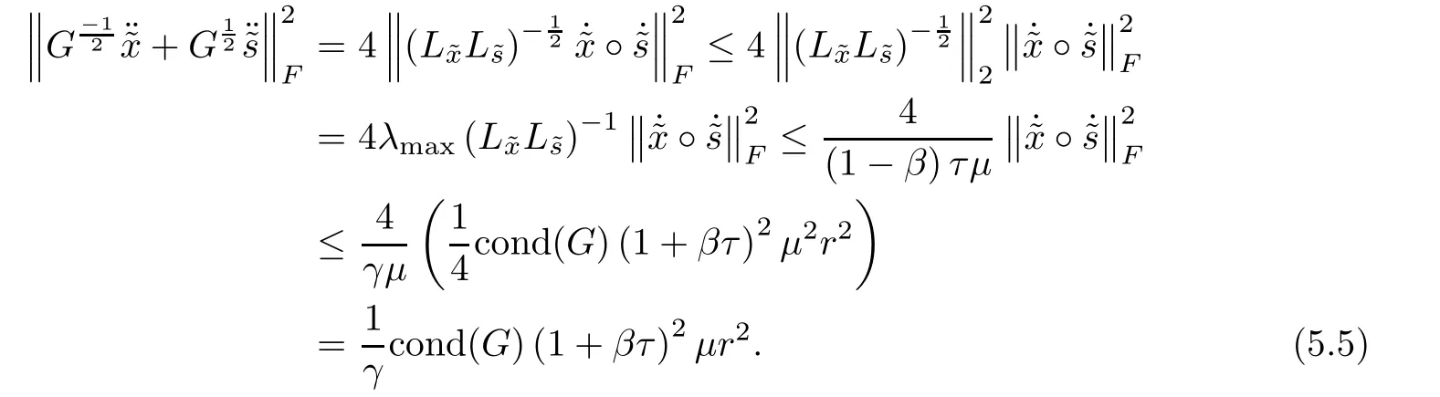
Substituting(5.5)into(5.4),the result is followed. ?

Proof Using Lemmas 5.6 and 5.2,we have

where the last inequality follows from Lemma 5.9.This follows the desired result. ?

Proof Due to Lemmas 5.6,5.2,5.8 and 5.10,we obtain

which implies(5.7).In the same way,inequality(5.8)is followed.This ends the proof. ?

ProofMultiplying the last equation of system(4.3)bytaking squared norm on both sides and using the fact trand Lemmas 5.6 and 5.2,we have

This gives the result.

In the same way as the proof of Lemmas 5.9 and 5.10,we derive the following result.

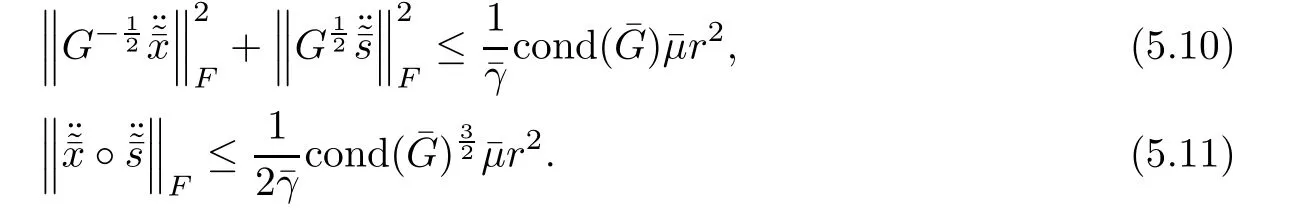
The following lemma is a direct result of Lemmas 5.12 and 5.13.

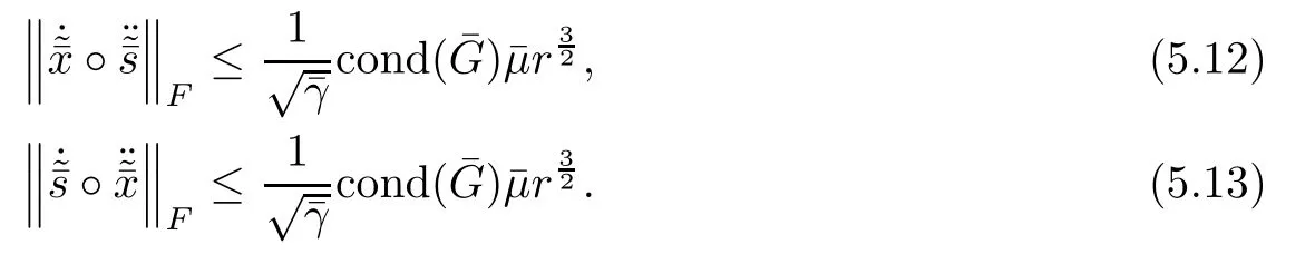
Proof The proof is similar to the proof of Lemma 5.11,and is therefore omitted. ?

6 Convergence Analysis

In this section,we present the convergence and complexity proof of Algorithm 1.First,we analyze the corrector step and show that,after a corrector step,the corrector point(x(ˆθ),y(ˆθ),Then,by analyzing the predictor step,we demonstrate the well-definition and convergency of the proposed algorithm.

6.1 Analysis of the Corrector-Step

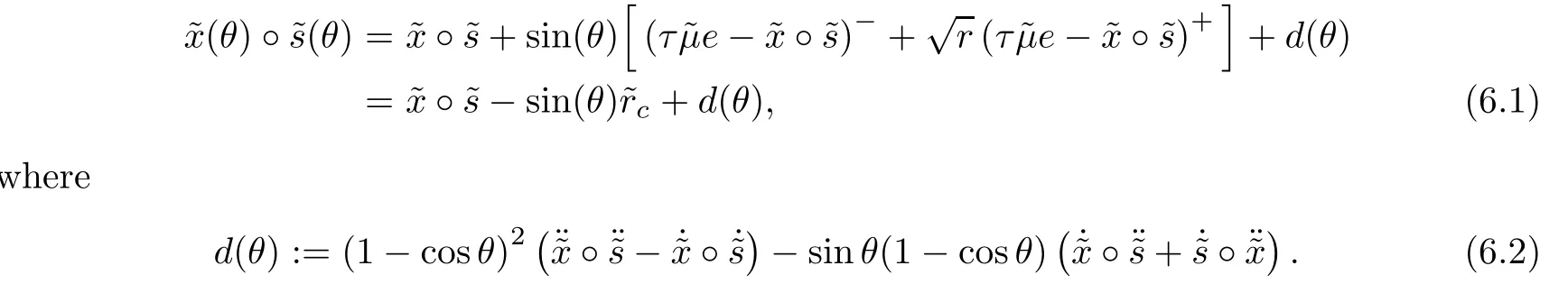
Clearly,due to systems(4.1)and(4.2),tr(d(θ))=0 and therefore

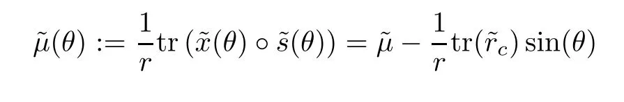
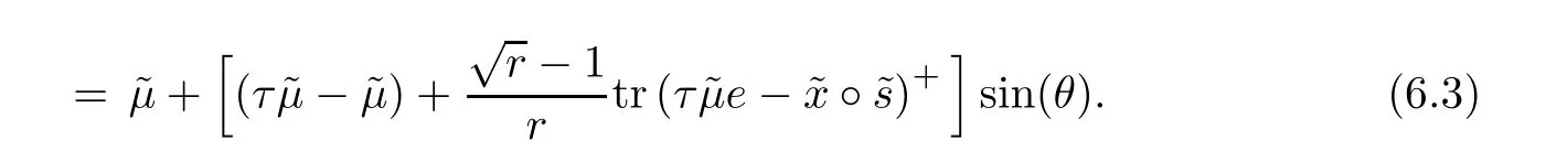
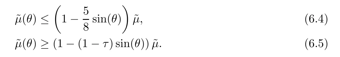
where the last inequality is due toMoreover,we derive

which implies(6.5)and completes the proof.

ProofDue to Lemma 6.1,we haveTherefore

where the first equality is due to the definition,the second inequality follows from Lemma 5.4 and the last inequality is due to the factsThe result is derived.?

The following lemma plays an important role in convergence analysis of the algorithm.

Lemma 6.3Let d(θ)be defined as(6.2)and sinThen

Proof Using Lemmas 5.8,5.10 and 5.11 and the fact 1 − cos(θ) ≤ sin2(θ)for θ∈ [0,],we derive

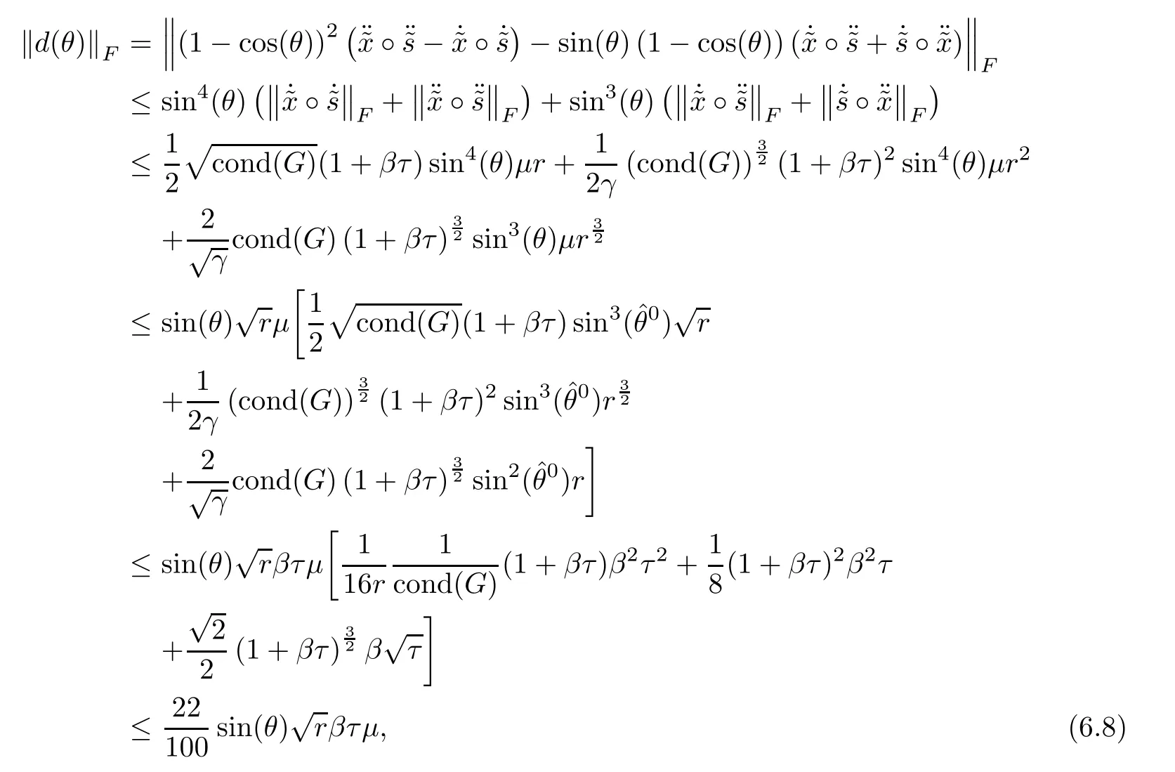
where the last inequality follows from τ≤,r≥ 4,β ≤and cond(G)≥ 1.This concludes the desired result. ?

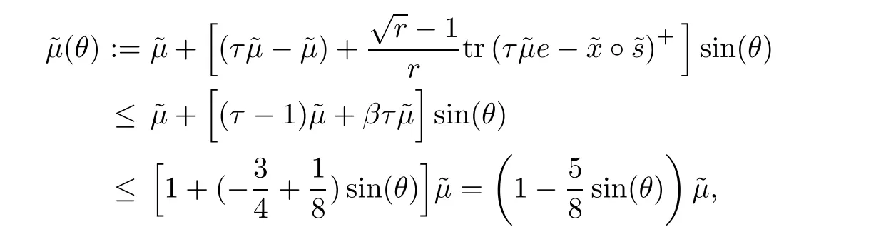
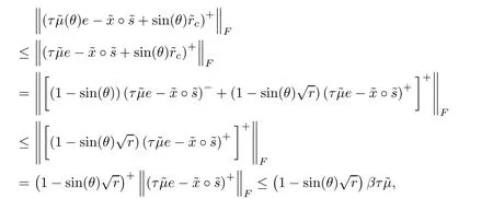
In the next lemma,we proceed to obtain an upper bound for the quantity β and show that after a corrector step the new generated point((θ),y(θ),(θ))belongs to the slightly smaller neighborhood NF(τ,).

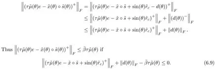
Using Lemmas 6.2,6.3 and 6.1,we obtain

which implies inequality(6.9)and therefore

On the other hand,using(6.10)and(6.5),we have

Finally,using Lemma 5.5 and(6.10),we conclude

The proof is completed.

6.2 Analysis of the Predictor-Step

After a corrector step,in order to further improvement of the optimality,the algorithm performs a predictor step.It considers the corrector pointas the starting point,calculates the predictor directionsby(4.3)and predictor2 and according to Lemma 3.1 computes the predictor pointas follows:

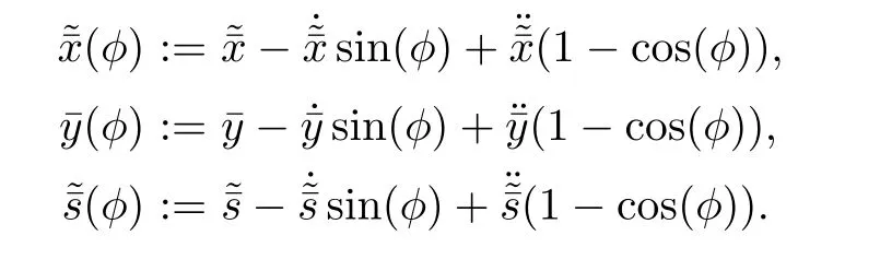
Thus,after a predictor step,we have

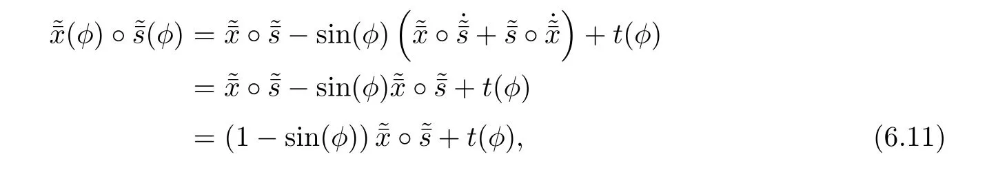
where

Clearly,using(4.3)and(4.4),tr(t(φ))=0 and therefore

In following,we analyze the predictor step in order to the predictor point( x(φ), y(φ), s(φ))∈NF(τ,β).Using Lemmas 5.12,5.13 and 5.14 and following the same proof as Lemma 6.3,we derive the following lemma.

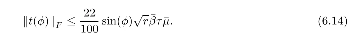
Lemma 6.5Let t(φ)be defined as(6.12)and

Then

The following lemma is the main result of this subsection.

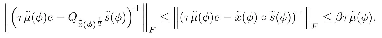
ProofFrom the definition NF(τ,β)in(3.6),we need to proveand the inequalityUsing(6.13)and(6.11),the inequality

or equivalently,using Lemma 5.4,

where the second last inequality is due toThis implies(6.15)and therefore

The later inequality,using(6.13),concludes

Finally,using Lemma 5.5 and(6.16),we conclude

This proves the lemma.

6.3 Polynomial Complexity

In this subsection,we prove the complexity bound of Algorithm 1.Due to the previous discussion,Algorithm 1 is well-defined and moreover after a predictor step we have

Now,we obtain some upper bounds for the quantity cond(·)for some specific search directions.

Lemma 6.7(Lemma 36 in[4])For the NT direction,cond(G)=1 while for the xs and sx directions,cond(G)≤where σ ∈(0,1)and r is the rank of J.

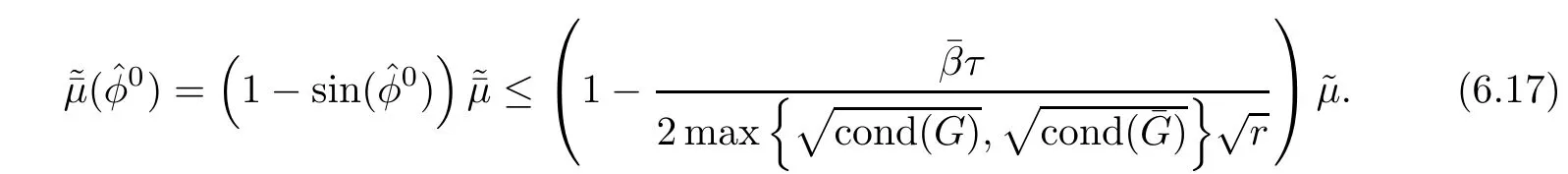
Using(6.17)and Lemma 6.7,we have the following result.

Corollary 6.8 If the NT search direction is used,the iteration complexity of Algorithm 1 is O(L)and if the xs and sx search directions are used,the iteration complexities of Algorithm 1 are O(rL).

7 Concluding Remarks

This paper proposed a corrector-predictor arc search interior-point algorithm for SO problems.Starting from an initial feasible solution and estimating the central path by an ellipse,the algorithm first performs a corrector step to improve both optimality and centrality.Then,in order to further improvement of optimality,the algorithm takes a predictor step and generates a new point in a slightly larger neighborhood of the central path.We proved that the proposed algorithm is well-defined and converges to an ε-optimal solution of the SO problem in polynomial time complexity.

AcknowledgementsThe authors also wish to thank Shahrekord University for financial support.The authors were also partially supported by the Center of Excellence for Mathematics,University of Shahrekord,Shahrekord,Iran.