
Lower bound estimation of the maximum allowable initial error and its numerical calculation
2018-12-07 09:28CAOYiXingZHENGQinndYANJun
CAO Yi-Xing,ZHENG Qinnd YAN Jun
aGraduate School,PLA Army Engineering University,Nanjing,China;bDepartment of Basic,PLA Army Engineering University,Nanjing,China
ABSTRACT In the numerical prediction of weather or climate events,the uncertainty of the initial values and/or prediction models can bring the forecast result’s uncertainty.Due to the absence of true states,studies on this problem mainly focus on the three subproblems of predictability,i.e.,the lower bound of the maximum predictable time,the upper bound of the prediction error,and the lower bound of the maximum allowable initial error.Aimed at the problem of the lower bound estimation of the maximum allowable initial error,this study first illustrates the shortcoming of the existing estimation,and then presents a new estimation based on the initial observation precision and proves it theoretically.Furthermore,the new lower bound estimations of both the two-dimensional ikeda model and lorenz96 model are obtained by using the cnop(conditional nonlinear optimal perturbation)method and a pso(particle swarm optimization)algorithm,and the estimated precisions are also analyzed.Besides,the estimations yielded by the existing and new formulas are compared;the results show that the estimations produced by the existing formula are often incorrect.
最大允许初始误差的下界估计及数值计算
KEYWORDS Predictability problem;maximum allowable initial error;particle swarm optimization algorithm;Conditional Nonlinear Optimal Perturbation(CNOP)
1.Introduction
In numerical weather and climate prediction,the prediction result is uncertain due to the uncertainty of initial values and models.Accordingly,Lorenz(1975)classified predictability problems into two types:the uncertainty of the forecast results caused by the initial conditionalerror,and thatby the modelerror.Numerical weather prediction is essentially initial and boundary problems of partial differential equations(Kalnay 2002),and initial values are generally provided by observations or background values.The initial error is inevitable because of the precision of observing instruments,discretization errors of the model,data loss in the initial value pretreatment,and so on.In addition,the absence of descriptions of some physical processes,and errors in certain parameters can make the model inaccurate and imperfect when describing atmospheric or oceanic movements,and then model error occurs.
Mu,Duan,and Wang(2002)divided predictability problems into three subproblems:problems associated with the maximum predictable time,prediction error,and the maximum allowable initial error(and parameter error).Since the true atmospheric value is not available in the actual numerical weather prediction,the quality of observations can be controlled within a certain range of precision,although there exists error between the initial value and true value.Taking these factors into account,Mu,Duan,and Wang(2002)further reduced the three subproblems into the lower bound of the maximum predictable time,the upper bound of the prediction error,and the lower bound of the maximum allowable initial error.Although estimations of these three subproblems are lower or upper bounds,they are of great guiding significance for the actual numerical weather prediction.
In studying the three reduced predictability subproblems,the programming of numerical experiments has always been an important issue because the related numerical results are indispensable.In previous research on the three predictability problems,some numerical experiments were based on the filtering method(Mu,Duan,and Wang 2002),i.e.,solving the objective function value at each mesh point by dividing the feasible region by an equal cube mesh.However,this method is only applicable to theoretical studies of simple models.As the division intervals decreases,the calculation amount increases sharply(Duan and Luo 2010)and cannot be realized in complexmodels.ConditionalNonlinear Optimal Perturbation(CNOP)is a kind of initial perturbation that satisfies some constraints and has the largest nonlinear evolution at the prediction moment.For predictability problems,CNOP is the initial error that leads to the maximum prediction error at the prediction moment(Mu and Duan 2003).Considering the physical meaning of CNOP,Duan and Luo(2010)firstly applied the CNOP method to solve the upper and lower bounds.Further,Zheng et al.(2017)gave a lower bound of the maximum predictable time and the upper bound of the prediction error by combining a particle swarm optimization algorithm(PSO)with CNOP.
There are many studies on the first and second subproblems,but few on the third.In particular,based on the existing lower bound estimation of the maximum allowable initial error,although the prediction error of the initial analysis always satisfies the limitation of the prediction error at the given prediction time,it is not a correct estimation.This study attempts to present a lower bound estimation and validate it theoretically and numerically.
The paperisorganized asfollows:Section2 describes the three predictability problems,giving a lower bound estimation of the maximum allowable initial error and its proof.Section 3 investigates the definition of CNOP and the two forecast models.In Section 4 we compare the performances of the two estimations in the two-dimensional Ikeda model and Lorenz96 model.A conclusion and discussion are presented in Section 5.
2.Three problems of predictability
This paper assumes that the model is perfect.What we focus on is the initial error,while ignoring the errors of the parameter.That is to say,denote Mtas the propagator that propagates the state from the initial time to time t;andare the true values of the state at the initial time and time t,respectively;then,).Norm ‖·‖Ais 2-norm in this paper.
Problem 1.Assume that the initial analysisis known and Mtis the propagator that propagates the state from the initial time 0 to time t.For any given prediction error ε>0,we call prediction T the allowable prediction time if

Mu,Duan,and Wang(2002)defined the maximum predictable time:
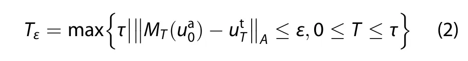
where τ is allowable prediction time.
Since the true value cannot be obtained exactly,it is impossible to obtain the exact value of Tεby solving this nonlinear optimization problem(Mu,Duan,and Wang 2002).When the initial analysis meets the quality control

a lower bound estimation of the maximum predictable time is given as(Mu,Duan,and Wang 2002)
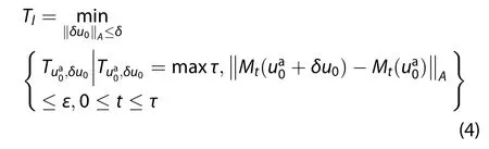
where δu0is initial perturbation.
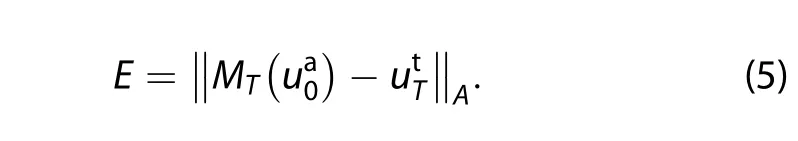
Similar to the above problem,it is also impossible to obtain the exact value of E.When the Equation(3)holds,an upper bound of prediction error(Eu)was given by Mu,Duan,and Wang(2002):
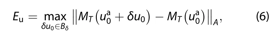
where Bδis a sphere with center at 0 and radius δ.
Problem 3.Assuming the initial analysisis known,for a given prediction moment T>0 and the allowable prediction error ε,the maximum allowable initial error is
Similar to the above problem,it is also impossible to obtain the exact value of the true state.If we know more information aboutthe errors ofuseful estimation can be derived.Suppose that the initial analysis holds that
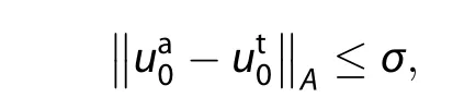
where the σ is the given constraint,then Mu,Duan,and Wang(2002)gave a lower bound estimation of the maximum allowable initial error:
and pointed out that

There are two points to note about the:
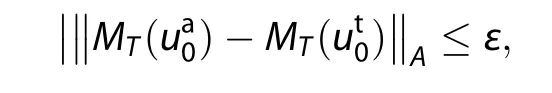
which means that the prediction error of the initial analysis at prediction moment T is less than the prediction error.
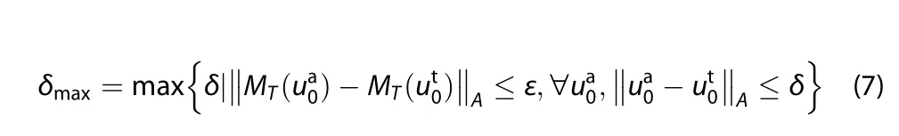
We give a lower bound of δmaxaccording to the definition of the maximum allowable initial error.Here is the estimation:
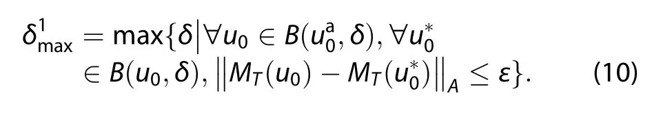
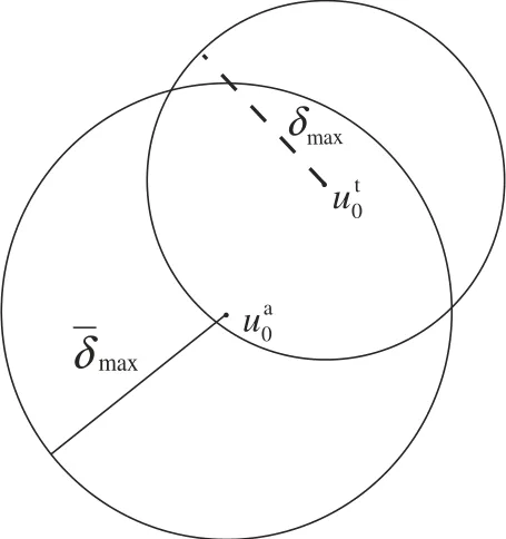
Figure 1.Interpretation of
From the Equation(10),we know that we have to search all the points around the points that are aroundThe calculation cost is so high that algorithms are difficult to design.
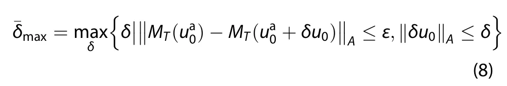
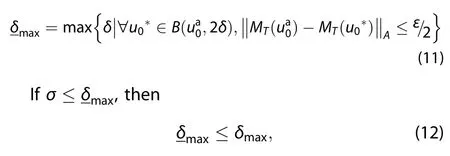
Considering Equation(10),it is easy to know that for anyThen,letsatisfyand considering the triangle inequality of norm,we know that for anyTherefore,we give another lower bound estimation
Proof:From Figure 2,we can easily see that for any
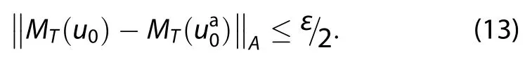

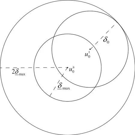
Figure 2.interpretation of
Combining with Equation(13)and the triangle inequality of norm,for any u0∈ B),
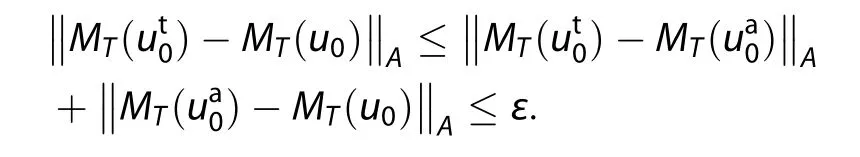
Combining with Equation(7)and Equation(14),we can imply that
Withoutmuch difficulty,we can prove that is less thanand is easy to solvewith the existing optimization algorithms.
3.Related concepts and the forecast model
3.1 Nonlinear model
3.1.1 Ikeda model
The Ikeda model was first proposed by Ikeda(1979).The description of the model in the next two paragraphs parallels that of Li,Zheng,and Zhou(2016).
The two-dimensional Ikeda model is adopted as the prediction model:
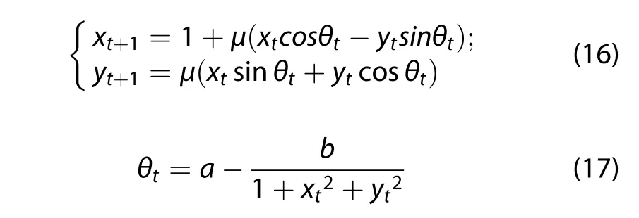
where 0 ≤ μ ≤ 1,a=0·4,and b=6.
From the expression of the model we find that there are trigonometric functions in Equation(16),and Equation(17)is a fraction whose denominator includes two quadratic components.Thus,the two-dimensional Ikeda model has fairly strong nonlinearity.
3.1.2 Lorenz96 model
The description of the model in the next three paragraphs parallels that of Wang(2007).
The Lorenz96 model is a new dynamic model derived and simplified from the dynamic model of Lorenz(1996).The model still has the characteristics of the Lorenz model and is very sensitive to the initial value.
The control faction of the model is
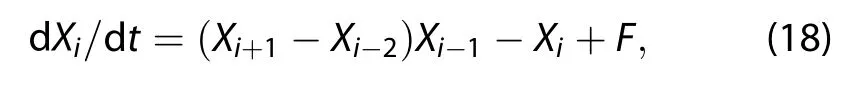
where i=1,2,···,N(N=40).Xiis the state of the system,and F is a forcing constant,and F=8 is a common value known to cause chaotic behavior.This model is solved using a fourth-order Runge–Kutta difference with a time step dt of 0.05 dimensionless units,equivalent to a time scale of 6 h in the real integration model.
3.2 CNOP
CNOP was proposed by Mu and Duan(2003)to study numerical weather and climate predictability and indicates a kind of initial perturbation that makes the maximum prediction error under certain constraints.The formula is the same as it in Mu and Duan(2003).
Denote M as a propagator and the initial value U0as a state vector.Integrate U0using M from the initial time to time t.For a given norm ‖·‖A,we call an initial perturbationa CNOP if and only if
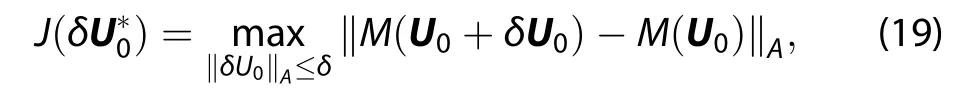
where δ is the given constraint of the norm ‖·‖A.
So far,the three predictability problems of the second part can be solved by solving CNOP.In the algorithm selection of solving CNOP,Zheng et al.(2017)compared the advantages and disadvantages of a traditional gradient algorithm and PSO in finding the CNOP and concluded that the PSO method can capture the CNOP more accurately.
In order to ensure that the obtained CNOP is accurate,when calculating the three predictability problems,we first look for the CNOP by using PSO to obtain the solution of the predictability problem,and then use thefiltering method to verify,which effectively shortens the calculation time.
4.Numerical experiments
Duan and Luo(2010)gave the calculation algorithm and gave the calculation flow chart.
In the numerical experiment reported in this paper,the predictiontimesaresetasT=5Δt,6Δt,7Δt,9Δt,and11Δt,and the maximum allowable prediction errors are E=0·5,0·8,1·1,1·4,and 1·7.
Table 1 demonstrates the calculations ofsolved by Equation(8).Table 2 demonstrates the calculations ofsolved by Equation(11).Table 1 is the same as in Yang,Zheng,and Wang(2017).
Table 1.Calculation results of
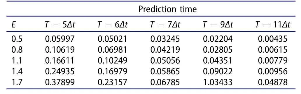
Table 1.Calculation results of
Prediction time E T=5Δt T=6Δt T=7Δt T=9Δt T=11Δt 0.50.059970.050210.032450.022040.00435 0.80.106190.069810.042190.028050.00615 1.10.166110.102490.050560.043510.00779 1.40.249350.169790.058650.090220.00956 1.70.378990.231570.067851.034330.04878
Table 2.Calculation results of
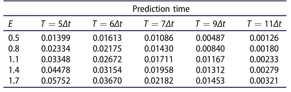
Table 2.Calculation results of
Prediction time E T=5Δt T=6Δt T=7Δt T=9Δt T=11Δt 0.50.013990.016130.010860.004870.00126 0.80.023340.021750.014300.008400.00180 1.10.033480.026720.017110.011670.00233 1.40.044780.031540.019580.013120.00279 1.70.057520.036700.021820.014530.00321
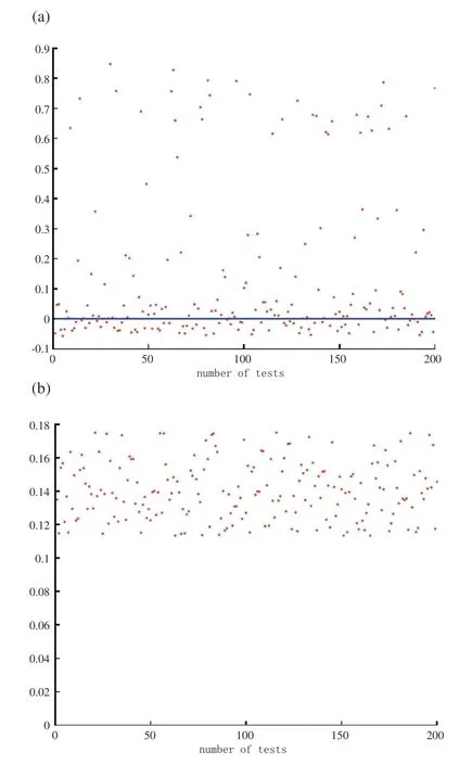
Figure 3.Results of(a)()and(b)(),when prediction error is 1.4 and prediction time is 6Δt.
None of the cases below the blue line satisfy Equation(11).It is clear from Figure 3 thatis not a lower bound estimation of δmax.The maximum allowable initial errors of the simulated true values are all more than=0·03154.In the 200 experiments,δmaxis in the range of 0.1450–0.2066 and its average value is 0.1718,whileis 18.36%of its average value.
For the Lorenz96 model,we use the following method to select the initial value:Firstly,a set of data is given.Then,we spin it up for 4000 days and select the result of one day randomly to spin up for another 365 days.Finally,we use the result of the 365th day as the initial value.When calculating the maximum allowable initial errors of the simulated true values,we set the prediction error as 3.0 and the prediction time as three days.When test and verifyandthe method to ensure the true value is the same as the Ikeda model.Figure 4 is the result.
None of the cases below the blue line(x-axis)satisfy Equation(11).The maximum allowable initial errors of the simulated true values are all more than=0·08570.In the 100 experiments,δmaxis in the range of 0.3224–0.3775 and its average value is 0.3498,whileis 24.50%of its average value.
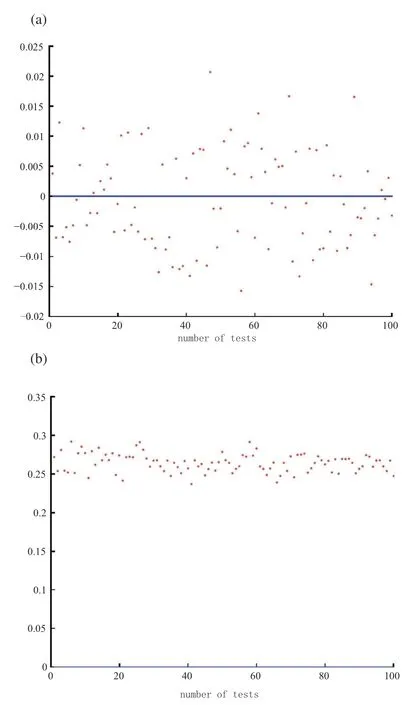
Figure 4.Results of(a)(δmax –)and(b)(δmax–).
It is clear from Figures 3 and 4 thatis not a lower bound estimation of δmaxandis a lower bound estimation of δmax.Althoughis not a lower bound estimation of δmax,it still plays an important role in practical applications.For the reason that for every initial value we can calculate itsand then compare it with the accuracy of the analysis value,if≥σ we can make sure that the prediction error of the initial value is good,which means the prediction error is less than ε.It is important to note,however,that the time and space of the calculation will increase because we have to do this for every initial value or observation.
5.Discussion and conclusion
Aimed at the third subproblem of predictability,we analyze the deficiencies of the existing lower bound estimation of the maximum allowable initial error.According to the definition of the maximum allowable initial error,a new lower bound estimation based on the initial observation is presented and proven.The numerical calculation of the new estimation is actualized by using the CNOP method and a PSO algorithm for both the Ikeda and Lorenz96 models.The estimations yielded by the existing and new formulas are compared to demonstrate the shortcomings of the existing estimation.
Subsequent work should try to make the estimation more accurate,study its relationship with the maximum allowable initial error in different and nonlinearly stronger models,and obtain the lower bound of the maximum allowable initial error more accurately.Also,considering the high-dimensional characteristicsofexisting climate modelsorweather models,it is worth exploring whether a PSO algorithm can perform well in high-dimensional optimization problems.
Disclosure statement
No potential conflict of interest was reported by the authors.
Funding
This work was supported by the National Natural Science Foundation of China(Grant No.41331174).
猜你喜欢
中学数学研究(江西)(2022年8期)2022-08-09
煤气与热力(2022年2期)2022-03-09
中学生数理化·高一版(2021年11期)2021-09-05
数学大世界(2021年10期)2021-06-05
内江师范学院学报(2021年4期)2021-05-06
舰船科学技术(2021年12期)2021-03-29
舰船科学技术(2021年12期)2021-03-29
智富时代(2018年5期)2018-07-18
智富时代(2018年5期)2018-07-18
数学学习与研究(2016年18期)2017-01-07
 Atmospheric and Oceanic Science Letters2018年5期
- Atmospheric and Oceanic Science Letters的其它文章
- Development of a global high-resolution marine dynamic environmental forecasting system
- Evaluation of the HadISST1 and NSIDC 1850 onward sea ice datasets with a focus on the Barents-Kara seas
- Subseasonal variation of winter rainfall anomalies over South China during the mature phase of super El Niño events
- Classification of wintertime large-scale tilted ridges over the Eurasian continent and their influences on surface air temperature
- Trajectory analysis of the propagation of Rossby waves on the Earth’s δ-surface
- Simulated and projected relationship between the East Asian winter monsoon and winter Arctic Oscillation in CMIP5 models