Numerical analysis of a magnetohydrodynamic duct flow with flow channel insert under a non-uniform magnetic field *

C. N. Kim

Department of Mechanical Engineering, College of Engineering, Kyung Hee University, Yong-in, Korea

Abstract: This study performs a numerical analysis of three-dimensional liquid metal (LM) magnetohydrodynamic (MHD) flows in a square duct with an FCI in a non-uniform magnetic field. The current study predicts detailed information on flow velocity, Lorentz force, pressure, current and electric potential of MHD duct flows for different Hartmann numbers. Also, the effect of the electric conductivity of FCI on the pressure drop along the main flow direction in a non-uniform magnetic field is examined. The present study investigates the features of LM MHD flows in consideration of the interdependency among the flow variables.

Key words: Non-uniform magnetic field, liquid metal blanket, magnetohydrodynamic (MHD) duct flow, flow channel insert

Introduction

For many years studies on self-cooled liquid metal blankets and dual-coolant lead-lithium (DCLL)blankets have been performed, where liquid metal serves both as breeder material and as coolant. Liquid metal flows therein have many merits, but are accompanied with problems and drawbacks caused by large pressure drop with a strong magnetic field and by degraded heat transfer with suppressed turbulence[1]. Therefore, the design of liquid metal flow should consider a minimized pressure drop and a proper velocity distribution enabling good heat transfer.

Numerous experimental studies[2-3]have been carried out to investigate the characteristics of magnetohydrodynamic (MHD) flows in ducts. Also,mathematical approach[4-5]has been performed to analyze the axial flow velocity in a cross section of a channel for fully developed flow under an applied magnetic field. And, three dimen- sional MHD flows based on computational fluid dynamics have been numerically analyzed in a straight duct with different codes developed by respective researchers with an aim to predict MHD flows accurately[6-14].

Piazza and Buhler[15]performed a numericalanalysis of buoyant MHD flows in differentially heated and internally heated ducts using CFX code.Also, with the same code Mistrangelo and Buhler[16]investigated liquid metal MHD flows in rectangular sudden expansions. These works showed that the numerical code gives accurate results up to the Hartmann number

Smolentsev et al.[17]numerically analyzed MHD flows and heat transfer in fully developed MHD flows with an FCI of SiCf/SiC in a poloidal channel of Dual Coolant Lithium Lead (DCLL) blanket. Here, they showed that the pressure drops with FCIs of the electric conductivities of 5 Ω-1m-1and 500 Ω-1m-1are 1/(200-400) and 1/10 times those without FCIs,respectively. Wong et al.[18]performed a numerical study on MHD flows with FCIs including slots and holes, showing that MHD flows with FCIs with holes yielded more notable side layer and M-shaped velocity distribution.

Smolentsev et al.[19]showed that high-velocity near-wall jets are observed near FCI walls when the electrical conductivity of FCIs are higher in US DCLL blanket channel with FCIs. Morley et al.[20]numerically investigated a developing MHD flow in the entrance region of an FCI in MHD channel when Hartmann number is 1 000. Zhang et al.[21], Wang et al.[22]numerically obtained fully developed MHD flows with FCIs in a straight duct, and reported that the acquired velocities are in good agreement with those obtained experimentally. Mao and Pan[23]performed numerical simulations of MHD effect in liquid metal blankets with an FCI with the use of two-dimensional fully developed flow model.Smolentsev et al.[24]carried out a numerical modeling of PbLi flow experiments in a rectangular duct with foam-based SiC flow channel insert. Smolentsev et al.[25]investigated MHD flows in a rectangular duct with non-conducting flow insert both in numerical and experimental method.

Though many studies have been performed about the effect of the FCIs on LM MHD flows, works on three-dimensional MHD flows in a duct with an FCI in a non-uniform magnetic field have not been performed much. This limitation may be attributed to the complexity in the nature of MHD flows.

In the current study, a mathematic model for three-dimensional MHD flows in a straight channel with an FCI in spatially changing magnetic field is to be numerically analyzed using CFX in consideration that the magnetic field intensity may spatially vary in a fusion blanket. Also, the effects of the Hartmann number and the electric conductivity of FCI on the MHD flow are to be investigated in detail, in consideration of the interdependency among the flow variables in LM MHD flows.

1. Problem formulation and solution method

1.1 Geometry, magnetic field and materials

The duct geometry considered in the study is given in Fig. 1, where a flow channel insert (FCI) is installed inside the channel wall. The cross-sectional dimensions are denoted in the figure. A narrow region of liquid metal is seen between the channel wall and FCI, and the slit is furnished in order to equalize the pressures of the fluids in the FCI and in the narrow region. The lengths of the channel wall and FCI are given to be 2.2 m, and a spatially varying magnetic field whose strength is expressed in the following equation is applied in the z direction (see Fig. 1(c)).

where0B is the characteristic magnetic field strength.

The values of electrical conductivities of the channel wall, FCI and liquid metal are given in Table 1. Basically, the analysis is performed forFGI=σ 500S/m with a magnetic field strength0=B 0.9623T, yielding the Hartmann number 1 000 based on the length scale of 0.05 m, the half- length of a side of the cross-section of the inner fluid region inside the FCI.

Fig. 1 (Color online) Duct geometry and applied magnetic field for MHD flows (mm)

Table 1 Material properties

1.2 Governing equations

In most practical liquid metal MHD flows, the magnetic Reynolds number is very small so that the induced magnetic field is negligible compared with the applied field. Therefore, the induction equation which governs the induced magnetic field will not be considered.

A steady-state, incompressible, constant-property,laminar flow of a liquid metal in the presence of a magnetic field is taken into account, and the system of equations governing this magnetohydrodynamic flow can be written as:

Conservation of mass

Equation of motion

Conservation of the charge

Ohm’s law

Substitution of Eq. (5) into Eq. (4) gives the following equation for the electric potential having elliptic behavior with a source term of the electromotive force.

Therefore, for a liquid metal magneto hydrodynamic flow, Eqs. (2), (3) and (6) are to be solved for the variables of the pressure, velocity and electric potential for the fluid part. For the electric features of the solid parts (the channel wall and FCI) only Eq. (6)is to be solved with zero source term (since u in the solid region is zero).

1.3 Boundary conditions

No slip condition is applied at the liquid-solid interface. At the inlet a uniform fluid velocity of =u 0.1 m/s is prescribed, and at the outlet the pressure is given to be zero.

The boundary condition for the electric potential is such that the whole system including the fluid,channel wall and FCI are electrically insulated from the outside, which can be written

at the inlet, outlet and outer wall of the channel wall.

1.4 Numerical method

The current study uses a structured grid system of 1 345 960 cells, which is chosen after a series of grid independency tests. Finer grids are employed in fluid region near the FCI and in narrow region (gap).Under-relaxation is employed in the iteration procedure in solving coupled governing equations. The second-order upwind scheme is used to discretize the convection terms, and the central difference scheme is employed for the diffusion terms. For the solution method of discretized equations, multigrid-accelerated incomplete lower upper factorization technique[26-27]is used. For the pressure-velocity coupling Rhie-Chow Interpolation method[28]is employed. For the validation and verification of the current numerical method Ref. [29] can be consulted.

2. Results and discussions

In the description about the current flow, it can be useful to distinguish the components in the right hand side of the general Ohm’s law so that =Jcan be expressed byThe first termdenotes the current induced by a local electric field (that is, by the gradient of electric potential), and can be called the electric-field component of the current (EFCC), while the second term J, means the current induced by a local fluid motion in a magnetic field,and may be referred to as the electro-motive component of the current (EMCC).

2.1 Near the inlet

In view of the electric conductivities given in Table 1, the induced current created in the vertical narrow fluid region can flow easily in the vertical narrow fluid region and in the vertical wall, while the existence of the FCI has a tendency to confine the current flow (created by the cross-product of the flow velocity and the magnetic field) to stay inside the FCI.Therefore, just behind the inlet, with considerable density of the current induced by the axial flow in the vertical narrow region, the Lorentz force therein can be considerable, reducing the axial velocity therein.

Therefore, the x-direction component of the pressure gradient (absolute value) in the vertical narrow region just behind the inlet is considerable near the inlet. Therefore, with a tendency of pressure equalization in most part of the axial region attained by the FCI slit, the pressure at the inlet of the vertical narrow region is quite higher (see Fig. 7). This is how the axial velocity in the vertical narrow region is steeply decreased just behind the inlet. This type of phenomenon is the outcome of the boundary condition of the uniform inlet velocity. In addition, in the top and bottom narrow region, because of the shape of the regions and the existence of FCI with low electric conductivity, the y-direction current component is smaller and the z-direction current component can be possible, leading to a smaller Lorentz force therein,yielding higher axial velocity therein.

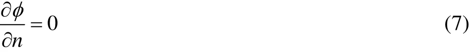
Fig. 2 (Color online)Featuresin the y-z planeat x =0.5m

F igure 2 s hows the features in the cross-sect ion of thechannelat x = 0.5 m , wheretheintensityof the magnetic field is not yet increased practically. In the vertical narrow regions and in most part of the inner flow region (inside the FCI), EMCC densityvectors head downward, as can be seen in Fig. 2(a), which is caused by the axial velocity(However, in fluid region near the slit smaller up ward EMCC vectors are observed, and below the slit the downward EMCC densities are weak. These will be explained later).

Since the EMCC flows downward in the crosssection in Fig. 2(a), a higher electric potential is induced in fluid region near the bottom surface (FCI wall) of the inner flow region, which yields the EFCC(=)σ φ-∇J in the y-direction. The induced EFCC and electric potential formed by the balance in the electromagnetic features are shown in Figs. 2(b), 2(c).

Inside the channel wall, the electric potential is near zero with a small spatial change because of its relatively high electric conductivity. Therefore, the EFCC in y direction is small in the vertical narrow region adjacent to the channel wall. Now, the distribution of the electric potential in the inner flow region is quite different. Because of the low electric conductivity of the FCI, highest electric potential is seen near the bottom surface of inner flow region,while lowest electric potential is observed near the top surface of inner flow region (especially, near the upper corners of the inner flow region). This type of electric potential distribution allows higher EFCC in the y-direction.

Figure 2(d) presents the closed loop of the current, the summation of the EMCC and EFCC. Here, the current that has passed through the slit mainly heads to each of the two upper corners of the inner flow region, where the lowest electric potential is observed. Then, it moves downward generally, gets across the FCI, and moves upward through the vertical duct walls. Some part of the current moves to the top duct wall to pass downward through the slit, and some other part moves down through the two vertical narrow regions.

Because of strong downward current flowing through the slit (see Fig. 2(d)) large Lorentz force is exerted in the negative x-direction near the slit,yielding negative x-directional velocity. In association with the applied magnetic field, this negative xdirection velocity induces upward EMCC (see Fig.2(a)).

The axial velocity in the y-z plane at =x 0.5 m is displayed in Fig. 2(e). Higher axial velocity is seen in the lower part of the inner flow region,while lower velocity is observed in the upper part,with the reverse flow near the slit. The axial velocity in the top and bottom narrow region is higher with negligible y-directional current therein, while that in the vertical narrow region is smaller because of the Lorentz force induced by the current in the negative y-direction therein.

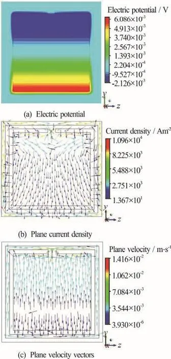
Fig. 3 (Color online) Features in the y-z plane at =1.0mx

2.2 In the region of changing magnetic field strength

The distribution of electric potential in the y-z plane at =1.0 mx is given in Fig. 3(a), where the peak value of the variable is higher than that observed at =0.5 mx . The density of the plane current in the cross-section is displayed in Fig. 3(b). In the upper part of the inner flow region, a pair of current recirculations are observed. Also, in the given cross-section the fluid comes into the inner flow region through the slit, as can be seen in Fig. 3(c). However, the absolute value of the velocity is very small.

The spatial change in the axial velocity in the region of increasing magnetic field intensity can be observed in Fig. 4. In general, the axial velocity in the lower part of the inner flow region is higher, while the axial velocity in the negative x-direction near the slit is notable. It is observed that as the fluid flows downstream, the axial velocity in the inner flow region generally increases, while that near the slot decreases to a higher negative value. It is related with an increase in the density of the current passing through the slot in association with a spatial increase in the magnetic field intensity.

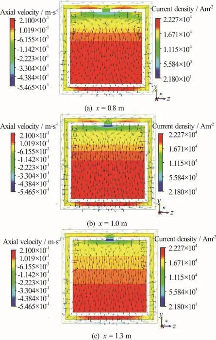
Fig. 4 (Color online) Axial velocities and current density vectors in several y-z planes in the region of spatially changing magnetic field strength

The velocity distribution in the mid x-y plane of the channel near =1.0 mx is shown in Fig. 5(a),depicting negative x-direction velocity near the slit and higher axial velocity in the lower part of the inner flow region (see also Fig. 4 depicting the axial velocity in several crosssections in the region of changing magnetic field strength).

Since the electric conductivity of the channel wall is rather high, the electric potential value in the channel wall is, in general, small. As shown in Fig.5(b), in the region of spatially changing magnetic field strength the current flows down obliquely in the negative x-direction in the top narrow region, passes downward through the slit, moves down obliquely in the positive x-direction in the upper part of the inner flow region, and flows down obliquely in the negative x-direction in the lower part of the inner flow region.This current would pass the bottom FCI wall, reach the bottom narrow region (and the bottom duct wall),move upward through the vertical duct wall, and arrive at the top duct wall, to form a large-scaled current loop. In the region of changing magnetic field intensity, the x-directional gradient of electric potential is negative in the upper part of the inner flow region, while that is positive in the lower part, as shown in Fig. 5(c). This makes the curved current path shown in Fig. 5(b).

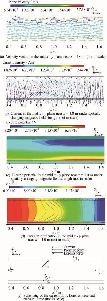
Fig. 5 (Color online) Spatial changes in variables in region of changing magnetic field strength (not in scale)

The pressure distribution is displayed in Fig. 5(d),where the equi-pressure lines are rather complicated.Based on the current flow shown in Fig. 5(b), a schematic of the relationship among the current,Lorentz force, and pressure force is depicted in Fig.5(e), where the pressure distribution can be estimated based on the fact that in an liquid metal (LM) MHD flow with higher Hartmann number, the Lorentz force induced by the current flow is approximately balanced with the pressure force. The pressure force estimated in Fig. 5(e) agrees well with that shown in Fig. 5(d).Based on the fact that the direction of Lorentz force is perpendicular to the plane current in the x-y plane,the streamlines of the current flow in Fig. 5(b) resemble the equi-pressure lines in Fig. 5(d)

2.3 Near the exit

In a region where the magnetic field intensity is not practically changing (say, at =2.0 mx ), the negative axial velocity is also observed near the slit as shown in Fig. 6(a). The general distribution of the electrical potential shown in Fig. 6(b) is similar to that obtained at =1.0 mx . However, the values of the electric potential are intensified due to higher magnetic field intensity, and therefore, the electric potential gradient in the y-direction is steeper than that at =0.1mx .

As shown in Figs. 6(a), 6(b), the spatial changes of the axial velocity and electric potential in the zdirection are very small or negligible. Also, the electromagnetic features are fully developed near the exit (for example, at x = 2.0 m ). Therefore, the axial velocity and electric potential in fluid region near the exit are a function of y only. Based on the above assumption, Eq. (6) can be reduced to

Integration of the above equation gives the following expression

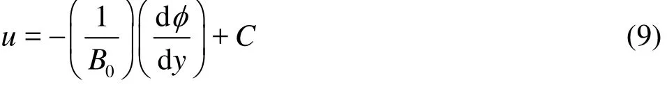
where the relationship between u andis derived. Now, Fig. 6(c) displays in detail the distributions of u andalong the yaxis (mid-z line) obtained in this study. The present numerical result is in a good agreement with the mathematical expression in Eq. (9) with a negligible value of C.

2.4 Pressure distribution

Fig. 6 (Color online) Features in the cross section near the exit(at =2.0mx )

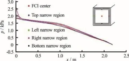
Fig. 7 (Color online) Distributions of the pressures along several imaginary lines in the channel

The distribution of pressures along several imaginary lines in the channel are depicted in Fig. 7,where in the region of low magnetic field intensity the pressures are decreased mildly, while in the region of high magnetic field intensity the pressures decrease steeply because of larger Lorentz force. The pressures in the narrows regions are, in general, a little bit higher than that at the slit. The pressure at the center of the inner flow region is almost the same as that at the slit in most part of the duct length, except in the region of changing magnetic field intensity where the former is a little bit higher than the latter, as also shown in Fig. 5(d). Note that the pressure at the exit is given to be zero. The rapid change of the pressure in the narrow region near the inlet has been addressed before.

Fig. 8 (Color online) Spatial changes in the pressures along the center of the channel with the electric conductivity of FCI 500 S/m for the Hartmann numbers of 500, 750 and 1 000

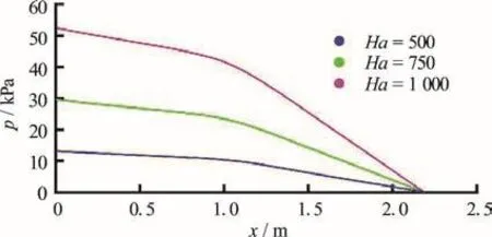
Fig. 9 (Color online) Spatial changes in the pressures along the center of the channel without FCI for the Hartmann numbers of 500, 750 and 1 000

2.5 Pressure drop depending on the Hartmann num-ber in cases with and without FCI

The effect of the characteristic magnetic field strength (or Hartmann number) on the pressure drop in the main flow direction for the FCI with the electric conductivity 500 S/m is displayed in Fig. 8. Here, the Hartmann numbers are evaluated based on the magnetic field intensity in the downstream. In general,the higher the magnetic field strength is, the larger the pressure drop is. Based on the current numerical result,the absolute values of the pressure gradients are examined in an axial region where the magnetic field strength is not changing practically. Here, the region of 1.5 m2.0 mx≤≤ is selected for the evaluation of the pressure gradients in consideration that the imposed boundary condition at the exit may affect the pressure gradients in the region of 2.0 m2.2 mx≤≤.For characteristic magnetic field strengths of 0.4816T,0.7244T and 0.9632T (corresponding Hartmann numbers of 500, 750 and 1 000, respectively), the pressure gradients are 286.5 Pa/m, 671.2 Pa/m and 1 065.7 Pa/m, respectively, and the nondimensionalized pressure gradients, are evaluated to be 0.01604, 0.01661 and 0.01492, respectively.

Also, the influence of the characteristic magnetic field strength (or the Hartmann number) on the pressure drop without FCI is depicted in Fig. 9. Similarly, the pressure gradients in the same region for the above three different field strengths are evaluated to be 9 228 Pa/m,20 690 Pa/m and 36 730 Pa/m, respectively. The comparison of the pressure gradients with and without the FCI shows that the installation of FCI of the electric conductivity 500 S/m can give a merit of reduced pressure drop with a factor of 0.0290 in case of the Hartmann number 1 000.

2.6 MHD flows depending on the electric conductivity of the FCI

The effect of the electrical conductivity of the FCI on the pressure drop in case of the Hartmann number 1 000 is displayed in Fig. 10. From this figure the pressure gradients can be obtained in a similar way.In the region of 1.6 m2.0 mx≤≤, for three different electrical conductivities of 25 S/m, 100 S/m, 500 S/m,the pressure gradients are 121.70 Pa/m, 295.4 Pa/m and 1 050 Pa/m, respectively, and the nondimensionalized pressure gradientsare 0.001703,0.004135 and 0.01470, respectively.

Fig. 10 (Color online) Effect of FCI electric conductivity on the pressure distribution

Also, in Fig. 10 the axial pressure forFCI=σ 100S/m is almost uniform in the region of 1.6 m≤increases therein in the direction of the main flow. As can be seen in Fig. 11, because the electric conductivities of the FCIs are quite small, the current induced in the inner flow region in the spatially changing magnetic field has a tendency to form a closed electric circuit in the inner flow region. This yields an upward component of the current flow in axial region of 0.4 m≤x≤0.9 m in the case o, and in 1.6 m2.0 mx≤≤ for. (However,this type of upward component of current is not observed in the case of, as seen in Fig. 5(b).) Now, the upward component of current yields Lorentz force in the x-direction, resulting in positive d/dp x. So, the flow is driven by the Lorentz force caused by upward current, while the pressure distribution opposes the flow. This type of flow can be called “current-driven flow”.

Fig. 11 (Col or online) Plane currents in the mid x-y plane nearx = 1.0munderspatiallychangingmagnetic field strengths (not in scale)

3. Conclusions

A numerical analysis for PDEs governing three-dimensional LM MHD flows with an FCI in a square duct in spatially changing magnetic field intensity has been performed. This study shows detailed features of the LM MHD flows in terms of the fluid velocity, current, electric potential and pressure.

In a situation where an FCI slit is located near the side wall of a duct, the slit used for the equalization of the pressures in the inside and outside of the FCI serves as a narrow passage through which the current flows in the axial regions of uniform, as well as spatially changing, magnetic field intensity. Because the induced current is stronger in the axial region of higher magnetic field intensity compared to that in the region of lower magnetic field intensity, the intensity of the current passing through the slit in the axial region of higher magnetic field intensity is higher.

Also, in the inner flow region inside the FCI, the values of the induced electric potential are higher in the axial region of higher magnetic field intensity compared to those in the region of lower magnetic field intensity. Therefore, a notable current in the axial direction can be induced, especially in cases with an FCI of very low electric conductivity, forming a closed electric circuit in the inner flow region. This yields the importance of three-dimensional effect in MHD duct flows in associated with spatially changing magnetic field.

Pressure drops in an MHD channel with and without FCI are evaluated for different Hartmann numbers, and the effect of the electric conductivity of the FCI on the pressure drop is addressed. The present study shows the interdependency among different flow variables of LM MHD flows including the electromotive component and the electric-field component of the current, which are directly connected with the liquid metal velocity and the gradient of electric potential, respectively.

Acknowledgements

This work was supported by the National R&D Program through the National Research Foundation of Korea (NRF) funded by the Ministry of Education,Science and Technology & Ministry of knowledge Economy (Grant No. 2015M1A7A1A02050613).