
A Scalable Method of Maintaining Order Statistics for Big Data Stream
2019-07-18 01:59ZhaohuiZhangJianChenLigongChenQiuwenLiuLijunYangPengweiWangandYongjunZheng
Computers Materials&Continua 2019年7期
Zhaohui Zhang* , Jian Chen, Ligong Chen, Qiuwen Liu, Lijun Yang, Pengwei Wang,2,3 and Yongjun Zheng
Abstract: Recently, there are some online quantile algorithms that work on how to analyze the order statistics about the high-volume and high-velocity data stream, but the drawback of these algorithms is not scalable because they take the GK algorithm as the subroutine, which is not known to be mergeable.Another drawback is that they can't maintain the correctness, which means the error will increase during the process of the window sliding.In this paper, we use a novel data structure to store the sketch that maintains the order statistics over sliding windows.Therefore three algorithms have been proposed based on the data structure.And the fixed-size window algorithm can keep the sketch of the last W elements.It is also scalable because of the mergeable property.The time-based window algorithm can always keep the sketch of the data in the last T time units.Finally, we provide the window aggregation algorithm which can help extend our algorithm into the distributed system.This provides a speed performance boost and makes it more suitable for modern applications such as system/network monitoring and anomaly detection.The experimental results show that our algorithm can not only achieve acceptable performance but also can actually maintain the correctness and be mergeable.
Keywords: Big data stream, online analytical processing, sliding windows, mergeable data sketches.
1 Introduction
The traditional application is built on the concept of persistent data sets that are stored reliably in stable storage and queried or updated several times throughout their lifetime [Zhang, Zhang, Wang et al.(2018)].Nowadays, large volumes of stream data arise rapidly,such as transactions in bank account [Zhang, Zhou, Zhang et al.(2018)] or e-commerce business[Yu,Ding,Liu et al.(2018)],credit card operations,data collection in Internet of Things (IoT) [Miao, Liu, Xu et al.(2018)], information in disaster management systems[Wu, Yan, Liu et al.(2015); Xu, Zhang, Liu et al.(2012); Wang, Zhang and Pengwei(2018)], behavior data analysis and anomaly detection in large-scale network service system [Zhang, Ge, Wang et al.(2017); Zhang and Cui (2017)] and data mining in live streaming[Li,Zhang,Xu et al.(2018)]etc.Analysis of order statistics plays an important role in analyzing data stream,which can help us to know the distribution of the data,make decisions, detect the anomaly data or help further data mining.Within applications, the high-volume and high-velocity features and limited memory make data stream pass only once,which means we can not store all the data in the memory and access the data that is already passed away.But if an approximate answer is acceptable, there are some online quantile algorithms that can maintain order statistics over data stream in the sketch and then we can get the approximate answer by querying the sketch.Combined with the sliding window, the online quantile algorithm can help us understand the order statistics or distribution of the recent data in the data stream.
In this paper, we propose a method that can maintain the data stream order statistics over the sliding window including fixed-size window and time-based window.A sketch will be created to store the stream data over the sliding window by our algorithm.Within a certain range of errors, we can get the result of quantile query or rank query from the sketch in a very short time.Compared to other algorithms that have been used to solve this kind of problem [Lin, Lu, Xu et al.(2004); Tangwongsan, Hirzel and Schneider (2018)],the advantages of our algorithm are the correctness-the error will not increase during the window updating and mergeable property-the sketches of two windows can be merged into one sketch.
And the remainder of this paper is constructed as follows.Section II introduces the related work that have been done till now.Section III gives some definitions that will be used in this paper and the basic data structure that we will use.Section IV represents our method to solve quantiles problem on the sliding window, including the basic structure,fixed-size window algorithm, time-based algorithm, and window aggregation.In section V, we designed some experiments to test the performance of our algorithm.And the last section V I gives conclusions of our work and describes the future work.
2 Related work
For the quantile problem, there are two surveys [Wang, Luo, Yi et al.(2013); Greenwald and Khanna (2016)] explain the status of research in terms of theory and algorithm in a very easy-to-understand way.In long-term research of quantile problem,there exist several algorithms to solve this problem.Greenwald et al.[Greenwald and Khanna(2001)]created an intricate deterministic algorithm(GK)that requiresspace.This method improved upon a deterministic(MRL)summary of Manku et al.[Manku,Rajagopalan and Lindsay (1998)] and a summary implied by Munro et al.[Munro and Paterson (1978)]which usespace.But Agarwal, et al.[Agarwal, Cormode, Huang et al.(2013)]prove that GK algorithm is not fully mergeable.Karnin et al.[Karnin, Lang and Liberty (2016)] created the optimal quantile algorithm as KLL, the best version of this algorithm requiresThe KLL algorithm is considered to be the optimal quantile algorithm until now both in terms of space usage.Considering the sliding window,Lin et al.[Lin,Lu,Xu et al.(2004)]was the first one to propose the quantile approximation solution in the sliding window model.And he achieved space usageArasu et al.[Arasu and Manku (2004)] improved this toThese algorithms are all based on the idea that split the window into small chunks and then use quantile algorithm to summarize each chunk.Yu et al.[Yu, Crouch, Chen et al.(2016)]proposed a sliding window algorithm called exponential histograms and used the GK algorithm as a subroutine, which is considered the best algorithm over sliding window until now, to the author's knowledge.But the approximation error will increase during the updating of the sliding window.For the window aggregation problem, a survey [Tangwongsan,Hirzel and Schneider(2018)]explain the theory and the current methods.Odysseas et al.[Papapetrou,Garofalakis and Deligiannakis(2012)]create a method can sketch distributed sliding-window data streams.
Considering the SW-GK is the optimal algorithm till now and it achieves great performance on the insert time and query time.But the drawback of this algorithm is that the window update way of SW-GK is to merge two structures and the approximation error will increase after each merge operation.The algorithms have been mentioned above take GK algorithm as a subroutine which is known don't have the mergeable property, so these algorithms can't aggregate different windows,which means they are not scalable.
3 Definition and model
3.1 Quantile and rank
Quantile and rank are both order statistics of data:the quantile φ(x)of a set N is an element x such that φ | N |elements of N are less than or equal to x.Given a set of elements x1,...,xn,the rank of x in a stream N as R(x) = φ | N |,which represents the number of elements such that xi≤x.And the quantile of a value x is the fraction of elements in the stream such that xi≤x.
In the ϵ-approximate problem,the data stream has N numeric elements.An additive error ϵn for R(x)is an ϵ approximation of its rank.In addition,when we query for a φ-quantile,where 0 ≤φ ≤1,we will get the result that is guaranteed to be in the[φ-ϵ,φ+ϵ]quantile range.
3.2 Sliding window
A data stream is a sequence of data elements available for a period of time.At any point in time,a sliding window over a stream is a bag of last W elements of the stream seen so far.To help us understand the recent data, we consider two types of sliding windows,the fixed-size sliding window whose window size is fixed and the time-based window whose window size varies over time.Formally,both types of windows are modeled using two basic operations-insert operation (insert a new element into the window) and delete operation(delete the oldest element from the window).
3.3 Basic structure
We firstly begin with the work of Karnin et al.[Karnin,Lang and Liberty(2016);Agarwal,Cormode,Huang et al.(2013)],which uses a special data structure to store the data over the whole stream.Here is the basic data structure of the algorithm-a compactor.A compactor can store k elements and each element has a weight of w.Different layer compactor has different capacity and weight.The compactor has a compaction operation, which can compact its k elements into k/2 elements of weight 2w.When the compactor finishes the compaction operation, we feed the results into the next layer compactor and so on.To maintain the order statistics and answer the quantile query, the requirement is that the elements in the compactor need to be in the order before compaction operation.During the compaction operation, either the even or the odd elements(based on the index)in the sequence are chosen.The unchosen elements are discarded,while the weight of the chosen elements is doubled.The error of the rank estimation before and after the compaction defers by at most w regardless of k.Fig.1 shows a simple example of a compactor, if its rank of a query in the compactor is even, the rank is unchanged.If it is odd, the rank is increased or decreased by w with equal probability.Fig.2 shows the structure of the compactors.The new element first comes to the first layer.When the first layer is full,compact the data in this layer and put the results into the second layer.When the second layer is full,do the similar operation and so on.
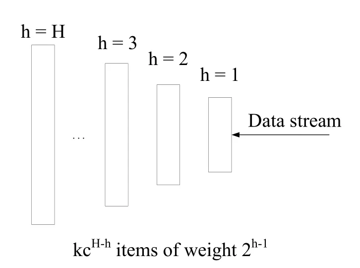
Figure 2: Compactors structure
We define the H as the numbers of layers of compactors and each compactor has its own capacity, denoted by khwith the indexes by their height h ∈1,...,H.The weight of elements at height h is wh= 2h-1.Considering the requirement of the compaction operation,the capacity of smallest compactor need be at least 2.For brevity,we set k =kH.It gives that kh≥kcH-hfor c ∈(0.5,1).
Lemma 3.1.There exists an algorithm that can compute an ϵ approximate for the rank or quantile problem whose space complexity isThis algorithm also produces mergeable summaries[Karnin,Lang and Liberty(2016)].
4 Method
4.1 Fixed-size window algorithm
For the fixed-size window, the insert operation is always combined with the delete operation.But we use the compactors to store the data,the element in different compactor has different weight with respect to the height, which means that one element doesn't represent itself, it has the weight, it records the number of compaction operation.So in the fixed-size window situation,we could not just delete the oldest element when the new element comes.Then we try to use a special array of size H to help to determine if it is the time to discard the oldest element in the sliding window.The index of this array is based on the height of the compactors.When the array of one layer count reaches to 2, turn on the trigger of this layer.When the trigger of the highest layer is on,it means it can discard the oldest element in the sliding window.
Here is the algorithm that we combine the insert operation and delete operation together.First, we have two conditions, one is that the current window is not full, which means we can continue to put the data into the window.Another is that the current window is full, which means the window sketch has represented W elements, with the new element comes,the oldest element should be discarded from the sketch.Note that the oldest element must be in the highest compactor, for example, kHrepresents the capacity of the highest compactor and wHrepresents the weight of the per element in the highest compactor.Our goal is to discard the oldest element in the window, according to the structure, when the new 2wHelements come in,theoretically,the oldest element in the sketch can be discarded.According to the compaction operation, for every layer, the data are in the order, we can compact the oldest element in this layer with its surrounding element(left or right with the same probability),so we use a H size array to trigger compaction operation.For the highest compactor,we pretend to do one compaction operation for the two elements-just deleting the oldest two elements.For other compactors,if the trigger is on,find the oldest element and its neighbor, discard one with the same probability and insert the other into the next compactor.In the end,update the trigger array.Note that the insert operation is finding the correct position to keep elements in the order in the compactors including insert operation on into the first layer.Fig.3 and Algorithm 1 describes the process of updating fixed-size window.For each layer, when the trigger is on, find the oldest element and its neighbor,discard one of them with equal probability and put the other into the next layer.For the last layer, after 2wHelements come, the trigger of this layer is on, discard the oldest two elements.The red circle represents the discarded one and yellow circle represents the one should be put into the next layer.

Algorithm 1 fixed-size window algorithm 1: procedure ADD(item)▷2:count ←count+1 3:if count <W then Sketch.update(item)4:else if count=W then 5:for h=0 →H do SortByValue(compactors[h])6:else 7:trigger[0]++8:for h=0 →H do 9:if h=H then 10:if trigger[h]=2 then 11:DeleteTwoOledst(h)12:else 13:if trigger[h]=2 then 14:One ←FindOldest(h)15:Two ←NearBy(One)16:if Random <0.5 then 17:Choose ←One 18:else 19:Choose ←Two 20:Delete(One,Two)21:Insert(h+1,Choose)22:trigger[h+1]++23:trigger[h]←0
Theorem 4.1.Our algorithm with W size window,has space complexitylog(ϵW)).And the update time complexity isand query complexity isThe correctness of our algorithm is unchanged, which can keep the rank query procedure still returns a value v with rank between(q-ϵ)W and(q+ϵ)W.
Proof.When the window is full,it means that this data structure is stable and this sketch represent W elements.Then we look at the data structure.
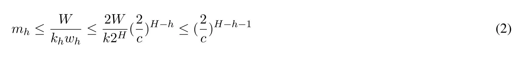
Firstly, we know that the second compactor from the top compacted its elements at least once.Therefore W/kH-1wH-1≥1 which gives

khrepresents the capacity of the compactor at height h and wh= 2h-1represents the weight of the per element in this compactor.Then we define mhto represent the number of compaction operations at height h.
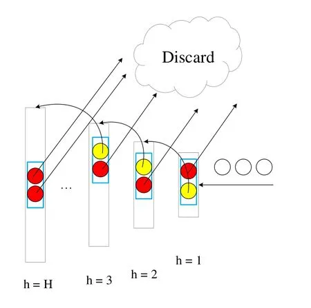
Figure 3: The process of updating fixed-size window
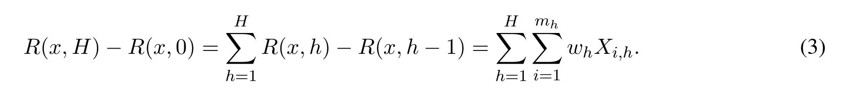
Then we use R(k,h) to represent the rank of x at height h.Note that each compaction operation in layer h either leaves the rank of x unchanged or adds wh or subtract wh with equal probability.Therefore,err(x,h) = R(x,h)-R(x,h-1) =where E[Xi,h] = 0 and |Xi,h|≤1.The final discrepancy between real rank of x and its our approximate rank=R(x,H)is
Lemma 4.1(Hoeffding).Let x1,...,Xmbe independent random variables, each with an expected value of zero,taking values in the range[-wi,wi].Then for any t >0,we got
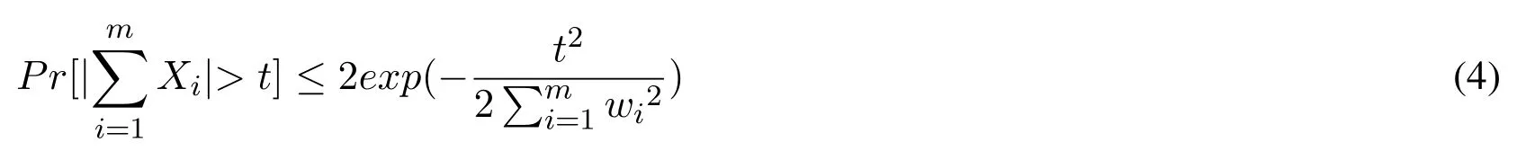
According to the Hoeffding's inequality,and we let ϵW be the total error.We can get the inequality below:
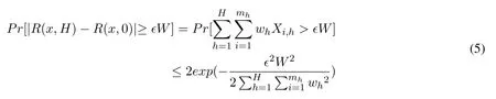
A computation shows that
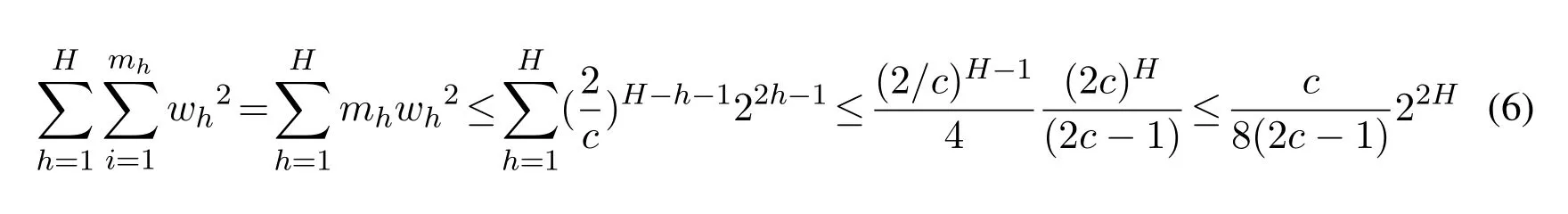
Substituting Eqs.(1)and(6)into Eq.(5)and setting C =(2c-1)c/4 we get the inequality

Note that the algorithm has H layers and kh≥kcH-h,c ∈(0.5,1),we let kh=「kcH-h⏋+1.In our algorithm,the total space usage includes two parts:the compactors and the trigger array,which is

According to Eq.(7)and requiring failure probability at most δ we conclude that it suffices to setThen we set δ =Ω(ϵ)suffices to union bound over the failure probabilities of O(1/ϵ)different quantiles.This provides a fixed-window algorithm for the quantiles problem of space
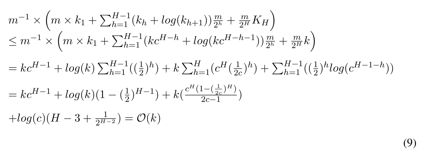
When the window is full, according to the algorithm, we can find that after two elements come, we need do one find oldest operation based on the time data arrives and one insert operation which inserts the chosen data into the next layer,which needs to find the correct position to make the elements in this layer are still in the order.In the first layer,we need to traverse the elements of this layer to find the oldest element and use binary search in the second layer to find the position to insert.After four elements come,there will be one find operation and one insert operation in the second layer and two find operations and two insert operations in the first layer, etc.What's more, we need also mention that inserting every element into the first layer also need to keep all the elements in the order in the first layer.So we can get the time cost per m elements,Based on the knowledgeand c ∈(0.5,1),the amortized time is According to the previous knowledge about k, we can get that the final update time complexity is
The query operation is to find all the elements stored in the compactors which are less than the given value and sum their weights together.Considering the compactors always contains the sorted elements,we could use the binary search to find the elements less than the given one,which gives the query time

Considering that H can be represent by thethe final query time complexity will be
During the execution of our algorithm, the height of compactors is not changed.Every compactor can have two more element at most and each compactor still leaves the rank of the x unchanged or add whor subtract whwith equal probability.For the layer h, the err(x,h)is unchanged.So the total error is stillThis means that our algorithm can maintain the correctness that the rank query procedure returns a value v with a rank between(q-ϵ)W and(q+ϵ)W .
4.2 Time-based window algorithm
For the time-based window,when a new item comes,put it into the first compactor.Then if the compactor is full, do the compaction operation.Based on the time the new item contains, compute the window threshold.Then do the delete operation, for every item stored in the compactors,if its time before the threshold,delete the item.
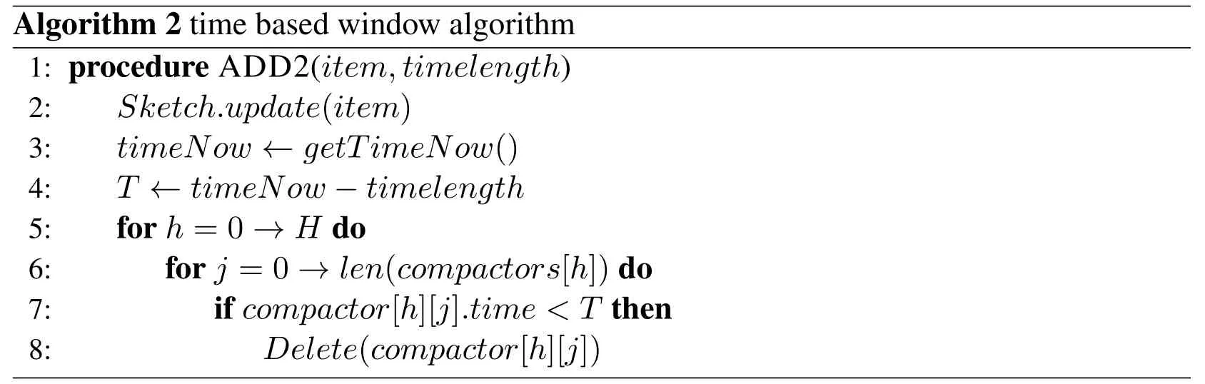
Algorithm 2 time based window algorithm 1: procedure ADD2(item,timelength)2:Sketch.update(item)3:timeNow ←getTimeNow()4:T ←timeNow-timelength 5:for h=0 →H do 6:for j =0 →len(compactors[h])do 7:if compactor[h][j].time <T then 8:Delete(compactor[h][j])
Theorem 4.2.Setting W′to the elements in the current time-based window,our algorithm with time-based window has update timeand query time
Proof.Note that every update operation needs traverse all the elements to delete the expired elements.The space usage isSo the update time isSimilarly, the query operation also need to traverse all the data,which givesquery time.
4.3 Window aggregation
Aggregating two windows means that merge the sketches of the two windows together.Firstly, let the small(the number of layer is small) one grow until it has at least as many compactors as the other.Then, Append the elements in same height compactors.Each level that contains more than khelements need do one compaction operation.

w aggregate algorithm 1: procedure AGGREGATE(s1,s2)2:if s1.height <s2.height then 3:s1.grow()4:else 5:s2.grow()6:for h=0 →H do 7:s1.compactor[h].add(s2.compactor[h])8:for h=0 →H do 9:if len(s1.compactor[h])>kh then 10:s1.compactor[h].compact
According to this mergeable property, we can extend our algorithm to the distributed environment, which can handle more huge data.Here is our distributed system structure,when the data comes,it will first come to the process point and then will be allocated to the different machines.Every machine uses our algorithm to sketch the stream data separately.Then merge all the sketches together.For example,if we want to analyze the data in the last 5 minutes.The data stream will be allocated to three nodes with Round-Robin Scheduling and every node only need to update 1/3 data.Then after every 30 seconds, we merge all the sketches into the final sketch.In this way, we can consider the final sketch maintains the order statistics of the last 5 minutes data.If we want to do some queries,we can get the approximate result from the final sketch.Fig.2.describes this system structure.For every window, the time resolution is 5 minutes.After every 30 seconds, we aggregate all the windows and get the final sketch.Then we query the final sketch for analyzing the order statistics of the recent 5 minutes.
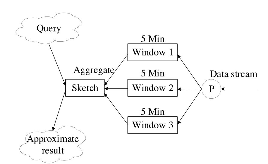
Figure 4: System structure.
5 Experiments
We mainly implemented our fixed-size algorithm by using Python and did some experiments to prove the performance of our algorithm.Experiments were run on a Core i5 2.1 GHz CPU computer with 8 Gb memory running Windows 10.The first experiment is a simple example to illustrate that our algorithm can really work.The second and third experiments are to test the insert operation and query operation time,separately.The fourth experiment is to calculate the storage that our algorithm need use.The fifth experiment is to prove the correctness of our algorithm,which means that the error between the real rank and the sketch rank will not increase during the process of the window sliding.The last experiment is to prove the mergeability of our algorithm.
5.1 A simple example
The parameters of our algorithm are k and W, where k is the maximum capacity of all compactors as we explained before and W is the window size.In this simple experiment,we set the k to 32 and W to 500.We use the Cumulative Distribution Function to describe the order statistics of the data.Fig.5 shows that the distribution of the last 500 elements,which are the end of the data stream.And Fig.6 describes the distribution generated by the sketch stored in our algorithm of the last 500 elements.Comparing Fig.5 and Fig.6,we can see that these two distributions are pretty similar,which means that our algorithm can actually maintain the order statistics over the sliding window.
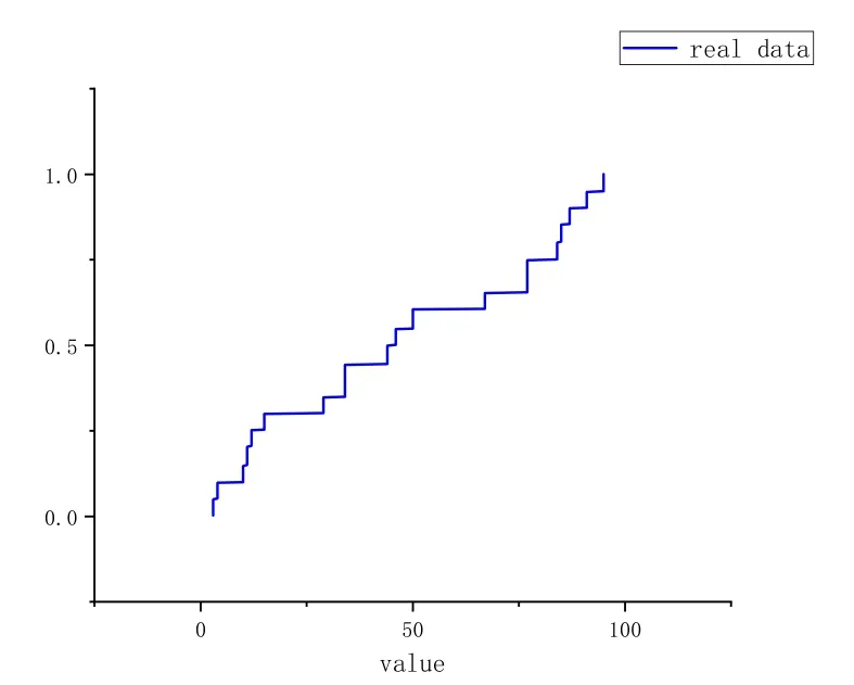
Figure 5: The CDF of the real data
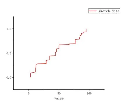
Figure 6: The CDF of the sketch data

Figure 7: The insert time

Figure 8: The query time
5.2 Insert time experiment
The previous section gives the insert time complexity by math derivation.In this section,we did an experiment to prove that the insert time is acceptable.We used a random dataset including 1000000 entries, set different parameters k and W and use this dataset to run our fixed-size sliding window algorithm.We calculate the running time as the insert time.In this experiment, we set different k, W and get different insert time.Fig.7 shows the relationship between the insert time and k and W.
From Fig.7,we can see that the insert time will rise with the increase of k and the window size doesn't have great influence on the insert time when the k is not big.But when k is set to 256 or much bigger, the influence of W will become longer.When the k is small,the insert time is pretty acceptable.Considering the window aggregation, we can extend our algorithm into the distributed environment,it will reduce the insert time dramatically.It means we can always control the insert time in a range that we want.
5.3 Query time experiment
Similarly, with the insert time experiment, we use the same dataset and the same parameters.After 10 elements,we query the rank or quantile of the value of the incoming element,then calculate the total query time.Fig.8 shows the result of the query time.
From Fig.8,when the k is set small the query operation is very pretty quick and not easily influenced by the window size.When the k is set large,the bigger window size has longer query time.
5.4 Sketch size experiment
From another point of view, the value of k determines the accuracy of the sketch, the greater the k value, the higher the accuracy, when the k become higher, the accuracy of the insertion time,query time,storage size will increase.Fig.9 describes the relationship between the sketch size and parameters k,W.The effect of k on storage size is greater than the value of W.For example,if we set k to 32,we may use approximately 100 elements to represent 1000 elements in the sliding window, even the window size increase to 100000 the storage size will increase to 125-a very small influence.
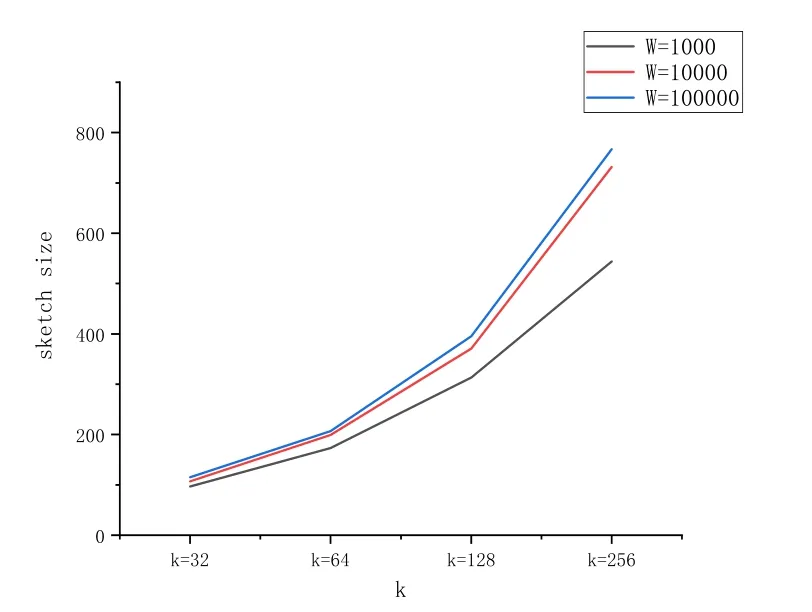
Figure 9: The sketch storage

Figure 10: The correctness test
5.5 Correctness experiment
The interesting part of our algorithm is that our algorithm can maintain the same correctness- the error will not increase during the process of the window sliding.This property has been proved in the previous section.Here is a simple example to illustrate this property,we set k to 128,W to 100000 and query the rank 1000 times during the process of the window sliding.We compare the real rank and our rank from the sketch and calculate the error between them.Fig.10 shows that the errors between real rank and our result during the 1000 queries.We can see the error is controlled in a certain range during the 1000 queries,which means the error did not increase during the process of the window sliding.
5.6 Window aggregation experiment
In the previous part, we have proposed the window aggregation algorithm, which means that the sketches of two windows can be merged into one window sketch.So in this section,we also implemented the window aggregation algorithm on our dataset.We split the stream data into two parts and each part runs one 500-size window algorithm.In the end, we merged these two sketches into one.We also use one program to run the 1000-size window algorithm.We also use CDF to describe the distribution of the data.Fig.11 describes the result of the 1000-size window algorithm and Fig.12 describes the result of the merged sketch of two 500-size window sketches.From Fig.11 and Fig.12,these two results are pretty similar and these two sketches can represent the distribution of the origin data.In this way,we also prove that our algorithm can actually be merged.

Figure 11: The CDF of 1000-size sketch
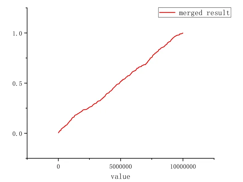
Figure 12: The CDF of merged sketch
6 Conclusions
In this paper,we propose a novel method that can maintain the stream data order statistics over the sliding fixed-size window, which can answer the quantile or rank query in a short time.The experiments show that our algorithm works properly and the insert time and query time are also both acceptable.Unlike other algorithms, our algorithm has the mergeable property and pay more attention to the correctness-the error will not increase during the process of the window sliding.
We also propose a time-based window algorithm, which is more flexible in different scenarios.In addition, the window aggregation algorithm enables parallel processing,which gives the opportunity to extend the quantile online algorithm into the distributed system.This provides a speed performance boost and makes it more suitable for modern applications such as system monitoring and anomaly detection.
For the future work,we are considering that if we accept the random method,the sampler is considered to be an effective method in the stream processing area.In the future,we are going to combine the sampler and our algorithm together to make further improvement in our algorithm.
Acknowledgement:This work was supported by National Natural Science Foundation of China(Nos.61472004,61602109),Shanghai Science and Technology Innovation Action Plan Project(No.16511100903)
 Computers Materials&Continua2019年7期
- Computers Materials&Continua的其它文章
- A DPN (Delegated Proof of Node) Mechanism for Secure Data Transmission in IoT Services
- A Hybrid Model for Anomalies Detection in AMI System Combining K-means Clustering and Deep Neural Network
- Topological Characterization of Book Graph and Stacked Book Graph
- Efficient Analysis of Vertical Projection Histogram to Segment Arabic Handwritten Characters
- An Auto-Calibration Approach to Robust and Secure Usage of Accelerometers for Human Motion Analysis in FES Therapies
- Balanced Deep Supervised Hashing