
Lump-type solutions of a generalized Kadomtsev–Petviashvili equation in(3+1)-dimensions∗
2019-11-06 00:42XuePingCheng程雪苹WenXiuMa马文秀andYunQingYang杨云青
Chinese Physics B 2019年10期
Xue-Ping Cheng(程雪苹), Wen-Xiu Ma(马文秀), and Yun-Qing Yang(杨云青)
1Physics,Mathematics,and Information College of Zhejiang Ocean University,Zhoushan 316004,China
2Key Laboratory of Oceanographic Big Data Mining&Application of Zhejiang Province,Zhoushan 316022,China
3Department of Mathematics and Statistics,University of South Florida,Tampa,FL 33620-5700,USA
4Department of Mathematics,King Abdulaziz University,Jeddah,Saudi Arabia
5College of Mathematics and Systems Science,Shandong University of Science and Technology,Qingdao 266590,China
6International Institute for Symmetry Analysis and Mathematical Modelling,Department of Mathematical Sciences,North-West University,Mafikeng Campus,Private Bag X2046,Mmabatho 2735,South Africa
Keywords:lump-type solution,generalized(3+1)-dimensional Kadomtsev–Petviashvili equation,Hirota bilinear form,symbolic computation
1.Introduction
The physical phenomena and processes that occur in nature generally have complicated nonlinear features.Nonlinear evolution equations,arising as the significant models for investigating the natural phenomena of science and engineering,appear in an extensive diversity of applications in solitary wave theory,hydrodynamics,meteorology,optical fibers,quantum mechanics,ocean engineering,plasma physics,condensed matter physics,and so on.Therefore searching for exact solutions of nonlinear evolution equations plays an important role in the analysis of these physical phenomena and engineering applications and has gradually become one of the most significant topic for both physicists and mathematicians.Up to now,a variety of exact nonlinear wave solutions for nonlinear evolution equations have been well constructed,including solitary waves,cnoidal waves,rogue waves,period waves,lump solutions,shock waves,compactons,peakon propeller solitons,as well as kinds of interaction waves.Among all these solutions,lump solutions have attracted a growing amount of attention in soliton theory in recent years,based on both theoretical predictions and experimental observations.[1–3]Lump solutions are a kind of analytical rational function solutions,localized in all directions in space. They can be used to describe nonlinear patterns on the surface of shallow water with dominating surface tension,[4,5]in plasma,[6]in nonlinear optic media,[7,8]in the Bose–Einstein condensation,[9,10]in thin elastic plates,[11]etc. From nice properties of lump solutions one can understand the shapes,amplitudes,velocities of solitons after the collision with other solitons.Till now,many researchers have studied lump solutions of different nonlinear equations.For instance,Gilson and Nimmo[12]presented lump solutions of the B-type KP(BKP)equation. Imai[13]found dromion and lump solutions of the Ishimori-I equation.Satsuma and Ablowitz[14]originated lump solutions in the two-dimensional(2D)nonlinear dispersive systems,Kaup[15]constructed the lump solutions for the three-dimensional(3D)three-wave resonant interaction.More recently,making full use of the symbolic computation software Maple,one of the authors(Ma)and his collaborators have offered plentiful of lump and lumptype solutions to various(2+1)-dimensional[(2+1)-D]and(3+1)-dimensional[(3+1)-D]nonlinear and linear equations,such as the KP equation,[16,17]the BKP equation,[18,19]the KP equation with a self-consistent source,[20]the(2+1)-D Ito equation,[21,22]the Hirota–Satsuma–Ito equation,[23]the generalized Bogoyavlensky–Konopelchenko equation,[24]the(2+1)-D extended KP equation,[25]the generalized Calogero–Bogoyavlenskii–Schiff equation,[26]the(3+1)-D Jimbo–Miwa equation,[27]the(3+1)-D linear PDEs,[28]the(3+1)-D nonlinear evolution equation,[29]and so on.
In this paper,we shall focus on a generalized(3+1)-D KP equation in the following form
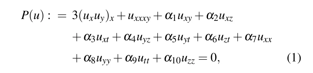
including all linear second-order derivative terms,where αi(i=1,...,10)are arbitrary constants.As the extended version of the KP equation,the generalized(3+1)-D KP equation(1)with αi(i=1,...,10)being random constants covers many specific equations(see the following paragraphs). In order to boost the possible applications of these equations in ocean studies and other fields,it is necessary to find analytical form of the lump-type waves for Eq.(1).As soon as the solution of the generalized(3+1)-D KP equation is given,the lump-type solution for all these specific equations can be acquired just by selecting different coefficients.
When α2=−3,α5=2,and the other αiare zeros,equation(1)becomes the(3+1)-D Jimbo–Miwa(JM)equation
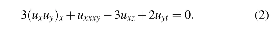
This equation was first introduced by Jimbo and Miwa in 1983.[30]It is the second member in the entire KP hierarchy,[31]which is used to describe certain interesting(3+1)-D waves in physics. The JM equation(2)has investigated regarding its solutions,non-integrability,and symmetries.The Painlevé method,the tanh-coth method,the simplified Hirota’s method,the extended homoclinic test approach,a transformed rational function method,and other methods were applied to obtain solitons,periodic,complexiton,lump-type solution,and travelling wave solutions to Eq.(2).[27,32–34]
While α3=α5=−α10=1,we have the generalized KP equation

Numerous studies have been conducted on extracting exact solutions and related properties to Eq.(3). For example,in Ref.[35],based on the Plücker relation and the Jacobi identity for determinants,Wronskian and Grammian formulations are established. Applying the proposed bilinear Bäcklund transformation,Ma and his collaborators have computed two classes of exponential and rational travelling wave solutions with arbitrary wave numbers.[36]Moreover, quasiperiodic waves,solitary waves,asymptotic properties,and rogue waves with interaction phenomena of Eq.(3)have been discussed in Ref.[37].
When α3=α5=α6=−α7=−α10=1,equation(1)reduces to the(3+1)-D BKP equation

which can be applied to describe the propagation of nonlinear waves in fluid dynamics.One-,two-,and multiple-soliton solutions for Eq.(4)have been discussed by Wazwaz.[38]Conservation laws for Eq.(4)have been constructed,along with some exact solutions.[39]Bilinear-form and Bell-polynomialform Bäcklund transformations for Eq.(4)have been presented,along with some soliton solutions as well.[40]On the basis of the bilinear equation of the(3+1)-D BKP equation,Zhao and Han[41]constructed its lump-type solutions by symbolic computation.
In Ref.[42],Ma applied the multiple exp-function algorithm to construct multiple wave solutions to the(3+1)-D generalized BKP equation

where the constants are chosen as α2=α5=−1.The resulting solutions involve generic phase shifts and wave frequencies.
Letting α3=α5=α6=−α7=−α8=−α10=1,we have the(3+1)-D generalized BKP equation

Wazwaz has established the one and two soliton solutions for equation(6)by using the simplified Hereman–Nuseir form.[38]
By taking α3=α5=α9=−α10=1,equation(1)turns into the(3+1)-D generalized KP–Boussinesq equation[43,44]

Kaur and Wazwaz[45]have explored lump solutions for Eq.(7)by reducing its(3+1)-D version into a(2+1)-D one,and they analyzed the sufficient and necessary conditions for assuring analyticity,positivity,and rational localization of the solutions at the same time.
If the coefficients are taken as α5=−1,α7=α10=−3,equation(1)becomes the generalized BKP equation

which is just the model investigated by Wazwaz et al.in Ref.[46],where the authors derived the multiple soliton solutions by the simplified Hirota’s direct method. Later,by making use of the same method,Wazwaz has also studied the multiple soliton solution for the generalized(3+1)-D KP equation[47]

In what follows,we begin with the Hirota bilinear form of the generalized(3+1)-D KP equation and make some assumptions by the superposition of quadratic functions to solve Eq.(1)in three cases of the coefficients in Section 2.To show the generality of the calculated lump-type solutions specifically,two representative ones are demonstrated in both analytical and graphical ways in Section 3.A summary and some discussions are given in the last section.
2.Abundant lump-type solutions
Generally,under the first-order logarithmic transformation

the generalized(3+1)-D KP equation(1)can be mapped into the Hirota bilinear form
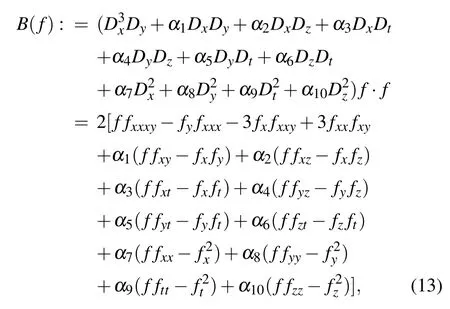
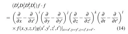
In fact,the actual relation between Eq.(1)and the bilinear equation(13)reads

and thus,if f solves the bilinear equation(13),then u=2(ln f)xwill present a solution of the generalized(3+1)-D KP equation(1).
The Hirota bilinear method allows us to establish Nsoliton solutions,[48]dromion-type solutions,[31,49]rational function solutions,[50,51]and so on,while in the present section,we would like to present lump-type solutions to the generalized(3+1)-D KP equation(1)based on its bilinear form(13).To search for lump-type solutions to the generalized(3+1)-D KP equation,we consider a trial solution for f in Eq.(13)as
with the wave variables
where all the parameters ai(i=1,...,16)are real constants to be determined.
Based on some inspections,we shall study the following three cases of solutions for the parameters αi:(i)α8=α9=0;(ii)α9=α10=0;(iii)α8=α10=0.In each case of solutions in the following list,the parameters not expressed in the set are arbitrary.Moreover,to simplify the mathematical expressions for solutions,we introduce some new constants as follows:

Case 1We first set α8=α9=0 for the generalized(3+1)-D bilinear equation(13). A direct substitution of the solution(16)with Eq.(17)into the bilinear equation(13)and a straightforward computation yield the following set of constraining equations on the parameters ai:
where

For simplifying the tedious expression of a16in Eq.(19),we did not write out the elaborate formulas for parameters a2,a4,a7,and a12in Eqs.(21)and(25)with ηi(i=1,...,10)shown in Eq.(18),which can be found from Eq.(19)with Eqs.(20)and(22)–(24).For f to be well-defined and positive,the involved parameters need to satisfy

Case 2We secondly consider the case α9=α10=0 for the generalized nonlinear equation(1).A similar direct computation generates the second solution set of the parameters:
where
The parameters a3,a8,a13,and a14arising in Eqs.(29)and(33)with Eq.(18)are given by Eq.(27)with Eqs.(28)and(30)–(32).Similarly,the involved parameters need to satisfy the conditions

to ensure that f is well-defined and positive.
Case 3Thirdly,we make α8=α10=0 for the generalized nonlinear equation(1).Using symbolic computation after a direct substitution of Eq.(16)with Eq.(17)into the bilinear equation(13)gains the following set of constraining equations on the parameters:
where
Here the parameters a2,a3,a7,and a12emerging in Eqs.(37)and(41)with Eq.(18)are all given by Eq.(35)with Eqs.(36)and(38)–(40).For f to be well-defined and positive,the involved parameters are required to satisfy the conditions

The above three sets of solutions for the parameters produce three quadratic function solutions to the bilinear generalized(3+1)-D KP equation(13)in three different cases:α8=α9=0,α9=α10=0,and α8=α10=0,respectively.Further,under the first-order logarithmic transformation(12),the resulting quadratic function solutions present three lumptype solutions u to the generalized(3+1)-D KP equation(1).In all three cases,the solutions contain eleven free constants ai,but always satisfy the determinant equation

Due to this character of the resulting parameters,it is obvious that all the above three solutions to the generalized(3+1)-D KP equation(1)are just lump-type solutions but not lump solutions.
3.Dynamics of two specific examples
In the current section,to show dynamic behaviors of the lump-type solutions more specifically,we would like to exhibit two special examples of the considered generalized(3+1)-D nonlinear equation(1),based on the lump-type solutions obtained above.
3.1.Example 1:Lump-type solutions to the BKP equation
Particularly,let us firstly focus on the BKP equation(4).For α8=α9=0 in Eq.(4),we may take into account its lumptype solution within the framework of Case 1.In fact,based on the free constants that not be constrained by Eq.(19),many different profiles of lump-type solutions can be designed.Just to avoid the tedious formula,we consider to fix these arbitrary constants at first. Associated with the eleven arbitrary wave parameters being selected as


the corresponding function f takes the form then a direct calculation from Eq.(12)tells us that the lumptype solution to the BKP equation can be expressed as

Under the parameters(44),b1=a8a11−a6a13=−20,the denominator of a2(or a7or a12)in Eq.(19)T1=90 and a16=2780/17>0,which guarantee the positivity of quadratic solution f and the analyticity of lump-type solution u. The graphical representation of the lump-type solution u of the BKP equation,shown by Eq.(46),is portrayed to illustrate the energy distribution of this solution in Fig.1,which includes contour plot,3D plot,and 2D curve.
As usual,we define the position of the maximum value and minimum value as the the peak and the trough of the lump-type wave.In the present case,according to solution(46),the peak and the trough are respectively located at
which reveals that the x values of both the peak and the trough of the lump-type wave change in proportion to z and time t,while the y value keeps invariant with time.The inserting of the coordinate values of the peak and the trough of the lump-type wave(47)and(48)into solution(46)resultsandThe result shows that both the peak value and the trough value are fixed constants,but not vary with t and z.As soon as z and t are given,the positions of the peak and the trough of the lump-type wave will be determined.If we select the mentioned values of free parameters as Eq.(44)and z=0,y=−45/391,and t={0,10,20},respectively,the peaks of the lump-type wave are respectively located at(3.85,−0.12),(−1.15,−0.12),and(−6.15,−0.12),while the trough are located at(−4.67,−0.12),(−9.67,−0.12),and(−14.67,−0.12),which have been depicted in Fig.1(c).

Fig.1.Lump-type profiles of Eq.(46):(a)contour plot with z=t=0;(b)3D plot with z=t=0;(c)the wave along with x axis with z=0,y=−45/391,and t={0,10,20},respectively.
3.2.Example 2:Lump-type solutions to the JM equation
By setting α2=−3,α5=2,and the other αiin Eq.(1)to be zeros,we have another specific example of the generalized(3+1)-D KP equation(2),i.e.,the JM equation.In the case α9=α10=0,associated with the parameters being taken as

the corresponding lump-type solution to the(3+1)-D JM equation can be written as

Figures 2(a)and 2(b)depict the contour plot and the 3D plot of the lump-type solution(50)of the JM equation,where the arbitrary constants are selected as Eq.(49)and z=t=0.Note that,under the circumstances,b4=a1a7−a2a6=−30,the denominator of a3(or a8or a13)in Eq.(27)T2=270,and a16=405/22>0 guarantee the quadratic solution f to be a positive solution and then the lump-type solution u to be analytical.
Continuing to choose the free constants as Eq.(49),we can compute from Eq.(50)that the peak and the trough are respectively located at


Different from the above results of BKP equation,both the x coordinate and y coordinate of the peak and the trough of the JM lump-type wave depend on z and t.After substituting the coordinate values(51)and(52)of the peak and trough into solution(50),we have

which tells us that the peak value and the trough value of the lump-type wave do not remain unchanged as that of the BKP lumptype wave,but vary with the changes of z and t.When we select the mentioned values of free parameters as Eq.(49)and z=0 and t={0,10,20},respectively,the peaks of the lump-type wave are respectively located at(−0.18,0.28),(−18.40,3.11),and(−35.95,5.93),while the trough are located at(−3.67,0.28),(−23.92,3.11),and(−44.85,5.93),and the maximum values and the minimum values of the lump-type solutions are(upeak,utrough)=({1.15,0.72,0.45},{−1.15,−0.72,−0.45}),respectively,which have all been displayed in Fig.2(c).
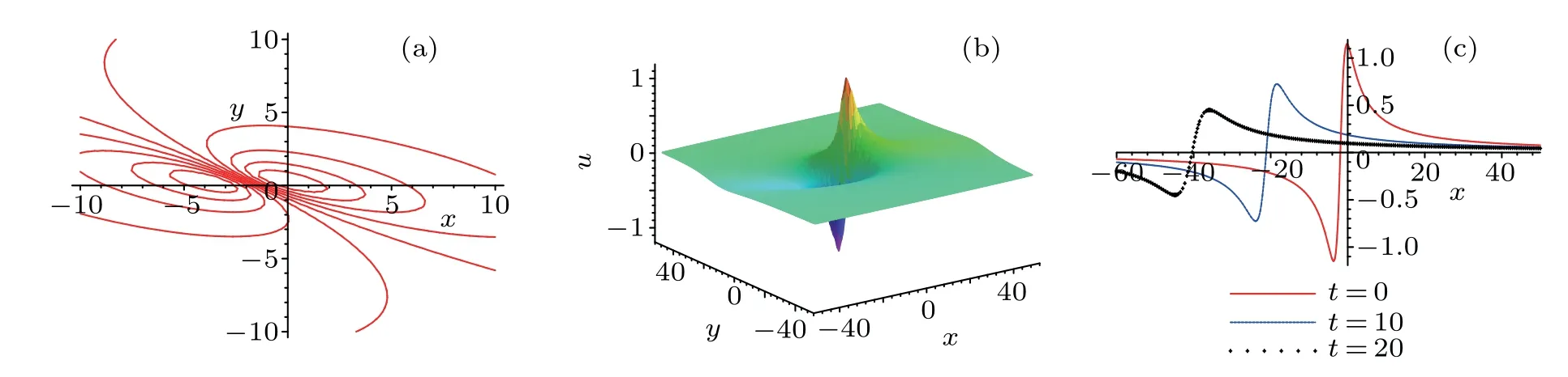
Fig.2.Plots of the lump-type solution(50)of the Jimbo–Miwa equation(2):(a)the contour plot with z=t=0,(b)the corresponding 3D plot with z=t=0,(c)the wave along with x axis with z=0,t={0,10,20},and y={0.28,3.11,5.93},respectively.
4.Summary and discussion
In this paper,on the basis of the Hirota bilinear formulation,we have investigated positive quadratic function solutions to a bilinear generalized(3+1)-D KP equation in three different cases. The resulting solutions offer us abundant new exact solutions to the corresponding nonlinear equation as well as some restriction conditions to ensure that the involved quadratic functions are well-defined and positive. More specifically,by considering two concrete nonlinear equations,the JM equation(2)and the BKP equation(4),we have illustrated the dynamical evolutions of the obtained lump-type solutions through their contour plots,3D plots and 2D plots with some certain choices of the included free parameters.Moreover,we have calculated the peaks and troughs of the acquired lump-type solutions as shown in Figs.1(c)and 2(c).It is worth stating that the implemented procedure can be applied to much higher dimensional nonlinear equations.It should also be interesting to consider interactions between lumps and solitons.[21,52]The details on the method for other nonlinear systems,other types of interaction wave solutions,and other possible physical applications,will be reported in our future research work.

- Chinese Physics B的其它文章
- Compact finite difference schemes for the backward fractional Feynman–Kac equation with fractional substantial derivative*
- Exact solutions of a(2+1)-dimensional extended shallow water wave equation∗
- Time evolution of angular momentum coherent state derived by virtue of entangled state representation and a new binomial theorem∗
- Boundary states for entanglement robustness under dephasing and bit flip channels*
- Manipulating transition of a two-component Bose–Einstein condensate with a weak δ-shaped laser∗
- Topological phases of a non-Hermitian coupled SSH ladder*