基于直线法MRLW方程的数值分析与模拟
2020-04-09 04:42邱玉婷
广州大学学报(自然科学版) 2020年5期
邱玉婷, 高 平
(广州大学 数学与信息科学学院, 广东 广州 510006)
0 Introduction
The generalized regularized long wave (GRLW) equation has the form:
Ut+Ux+p(p+1)UpUx-μUxxt=0
(1)
wherepis a positive integer,μis positive constant,tis time andxis the space coordinate. This equation has a major role in the propagation of nonlinear dispersive wave and many authors have investigated its numerical solution. Zhang[1]used finite difference method for a Cauchy problem of Eq.(1). Numerical solution of the GRLW equation has been obtained by Soliman[2]using He’s variational iteration method. Mokhtari et al.[3]presented the Sinc-collocation method for this equation. Roshan[4]obtained the numerical solutions of the equation with Petrov- Galerkin method using a linear hat function as the trial function and a quintic B-spline function as the test function. Akbari et al.[5]studied the equation using a compact finite difference method. The GRLW equation has been solved numerically by Karakoç et al.[6]using septic B-spline collocation method. A special case of Eq.(1) forp=1 is the regularized long wave (RLW) equation which is used to model a large number of problems in various areas of science. The equation was originally introduced to explain behavior of the undular bore development[7]. Until now, many researchers have solved the RLW equation by using various analytic and numerical methods. For instance, finite difference methods[8], mesh-free methods[9], Fourier pseudo-spectral methods[10]and various forms of finite element methods including collocation, Galerkin and least square methods (see Refs[11-13], for the details). In the present work, we consider another special case of Eq.(1) forp=2, the MRLW equation given by
ut+ux+6u2ux-μuxxt=0
(2)
with physical boundary conditionsu→0 asx→±∞. In this study, boundary and initial conditions are chosen
u(a,t)=0,u(b,t)=0
(3)
ux(a,t)=0,ux(b,t)=0
(4)
uxx(a,t)=0,uxx(b,t)=0
(5)
u(x,0)=f(x),a≤x≤b
(6)
wheref(x) is a localized disturbance inside the interval [a,b] and will be determined later. Various methods have been used for the numerical solution of MRLW equation, for instance B-spline finite element method[14-15], Adomian decomposition method[16]and collocation method[17].
In the present paper, we have applied MOL[18]to the MRLW equation. This work is built as follows. In Section 2, numerical scheme is explained. In Section 3, implementation of the method to Eq.(1) is explained. Numerical examples and results are given in Section 4. In Section 5, conclusion is presented.
1 The method of lines
The MOL is a numerical method for solving PDE problems that proceeds in two separate steps. First, spatial derivatives, e.g.,ux,uxx,…, are approximated using, for instance, finite difference(FD) or finite element(FE) methods; Second, the resulting system of semi-discrete ODEs in the initial value variable is integrated in timet. Obviously, an advantage of the MOL is that one can use all kinds of ODE solvers and techniques to solve the semi-discrete ODEs directly.
The MOL is considered as a special finite difference method but more efficient with respect to accuracy and computational time than the regular finite difference method. It essentially includes discretizing a given differential equation in one or two dimensions while using analytical solution in the remaining direction. MOL has the advantages of both the finite difference method and analytical method, it does not yield false modes nor the problem of relative convergence. The MOL has been used by many authors. It is used to find the numerical solution of the KdV equation[19]and nonlinear dispersive waves[20]. A generalization of the MOL for the numerical solution of the coupled forced vibration of beams presented in Ref.[21]. In any case, the MOL has the following properties that justify its use[22]:
(1)Computational efficiency. The semi-analytical character of the formulation leads to a simple and compact algorithm, which yields accurate results with less computational effort than other techniques.
(2)Numerical stability. By separating discretization of space and time, it is easy to establish the stability and the convergence for a wide range of problems.
(3)Reduced programming effort. By making use of the state of the art well documented and reliable ODEs solvers, programming effort can be substantially reduced.
(4)Reduced computational time. Since only a small amount of discretization lines is necessary in the computation, there is no need to solve a large system of equations, hence computing time is small.
To apply MOL normally includes the following five basic steps:
Step 1: Division the solution region into layers;
Step 2: Discretization of the differential equation in one coordinate direction;
Step 3: Transformation to obtain separated ordinary differential equations;
Step 4: Inverse transformation and insertion of the boundary conditions;
Step 5: Solution of the equations.
2 Implementation of numerical method
Let us subdivide the solution domain of the MRLW equationa≤x≤binto uniform rectangular mesh by the lines.
(7)
The MOL approximation of Eq.(1) intis based on the following finite difference approximation for the second derivative inx:

(8)
By substituting Eq.(7) and Eq.(8) into Eq.(2) and taking into account thatu1(t)=un+1(t)=0, the following system of ODEs is obtained:
(9)
(10)
(11)
This system can be written in the following form:
Aut(iΔx,t)=B
(12)
where
It can be easily solved by computingA-1, this yields a system of ordinary differential equations depending on the time variable in the form:

(13)
3 Numerical tests and results
To show the accuracy of the numerical scheme and to compare our results with both exact values and other results given in the literature, theL2andL∞error norms are calculated by using the analytical solution in Ref.[23]. Three test problems, including motion of a single solitary wave, interaction of two solitary waves and the Maxwellian initial condition, are investigated. Furthermore, three invariants[24]are calculated in order to show the conservation properties of the numerical scheme. The error normsL2andL∞are given as follows:
(14)
(15)
The exact solution of MRLW Eq.(2) given in Ref.[14] is
(16)
(17)
Three invariants of motion which correspond to conservation of mass, momentum and energy given in Ref.[14] are
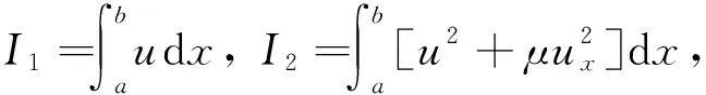
(18)
3.1 The motion of single solitary wave

We considerc=1, Δt=0.01, Δx=0.1 to compare our results with Refs[6, 15, 17], so the solitary wave has amplitude=1. The analytical values for the invariants areI1=4.442 88,I2=3.299 83 andI3=1.414 21. In order to find error norms and the invariant at different times, the computations are carried out for times up tot=18. The obtained results are reported in Table 1 which shows that three invariants are almost constant as the time progresses. Moreover, Table 2 represents the values of the invariants and error norms of the present method atT=6 against the results of Karakoç et al.[6], Raslan et al.[15], Khalifa et al[17]. We find that our scheme provides better results than others. Solitary wave profiles are depicted at different time levels in Fig.1 in which the soliton moves to the right at a constant speed and nearly unchanged amplitude as time increases, as expected.

Table 1 The invariant and the error norms for single solitary wave with amplitude=1, c=1, Δt=0.01, Δx=0.1, μ=1, 0≤x≤100

Table 2 The invariant and the error norms for single solitary wave with amplitude=1, c=1, Δt=0.01, Δx=0.1, μ=1, 0≤x≤100, T=6

Fig.1 Single solitary wave solution with c=1, x0=40, 0≤x≤100 at t=0, 6, 12, 18
3.2 The interaction of two solitary waves
We consider interaction of two solitary waves using the following initial condition in Eq.(2):
(19)

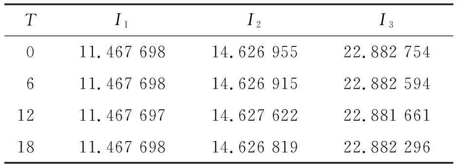
Table 3 Invariant of interaction in three solitary waves of MRLW equation, c1=4, c2=1, x1=-15, x2=25, Δt=0.01, Δx=0.1, μ=1, -50≤x≤200
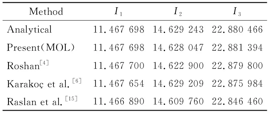
Table 4 Invariant of interaction in three solitary waves of MRLW equation, c1=4, c2=1, x1=-15, x2=25, Δt=0.01, Δx=0.1, μ=1, -50≤x≤200, t=8

Fig.2 Two solitary waves with c1=4, c2=1, x1=-15, x2=25 and μ=1 in the interval [-50, 200]
3.3 The Maxwellian initial condition
In the final test problem, the evolution of solitary waves is studied by using the Maxwellian initial condition:
u(x,0)=e-(x-40)2, 0≤x≤100
(20)
In this case, the behavior of the solution depends on the values ofμ. Therefore, we chose the values ofμ=0.1, 0.04, 0.015 and 0.005. The numerical computations are done up tot=18. The values of the three invariants of motion for differentμare presented in Table 5.

Table 5 The invariant for Maxwellian initial condition


Fig.3 Maxwellian initial condition at t=12; (a) μ=0.1, (b) μ=0.04, (c) μ=0.015, (d) μ=0.005
4 Conclusion
In this paper, the method of lines is used to simulate modified regularized long wave equations. The method is validated by choosing three test problems from literature. The accuracy of the method is examined throughL2andL∞error norms and the invariant quantitiesI1,I2andI3. It has been observed that the error norms are sufficiently small and the invariants are almost constant and almost coincide with their exact values during the simulation. All numerical results have been represented by figures and tables at different time levels. Advantages of the method are that it is easy to use and gives accurate solutions with little computational effort. With few modifications, the method can be employed to solve a number of different partial differential equations. Also the numerical procedure described in the paper demonstrates the ease with which the MOL can be applied to the solution of PDE using established numerical approximations implemented in library routines.
猜你喜欢
山西大同大学学报(自然科学版)(2022年1期)2022-03-17
房地产导刊(2021年12期)2021-12-31
房地产导刊(2020年11期)2020-12-28
美与时代·城市版(2020年6期)2020-09-15
美与时代·城市版(2020年6期)2020-09-15
房地产导刊(2020年7期)2020-08-24
中学数学研究(江西)(2020年7期)2020-07-22
小读者(2020年4期)2020-06-16
美与时代·城市版(2019年4期)2019-05-24
中国科技期刊研究(2016年11期)2016-04-17