Influence of different parameters on numerical simulation of vertical-axis marine current turbine based on OpenFOAM
2020-05-13 10:27,*,,,,
排灌机械工程学报 2020年4期
, *, , , ,
(1. College of Shipbuilding Engineering, Harbin Engineering University, Harbin, Heilongjiang 150001, China; 2. Institute of Ocean Renewable Energy System, Harbin Engineering University, Harbin, Heilongjiang 150001, China; 3. College of Energy and Electrical Engineering, Hohai University, Nanjing, Jiangsu 211100, China)
Abstract: Using the PimpleDyMFoam solver in open-source computing software OpenFOAM, based on the SST k-ω turbulence model and PIMPLE algorithm, a numerical simulation method of vertical-axis marine current turbines(VMCTs) is proposed, and the calculated results are compared with the experimental results. The results show that the numerical simulation method is feasible. Compared with other commercial softwares, this method has the advantages of higher solution efficiency and greater flexibility. According to the needs of users, the solver can be built on the basis of original code, and the corresponding discrete method can be optimized. This method can achieve optimization algorithms, save time and cost, etc. Secondly, the effects of different parameters (mesh density, time step, the selection of sidewall boundary conditions and inlet turbulence intensity) on numerical simulation of the VMCT are studied in detail. The findings summarize an effective CFD simulation strategy based on OpenFOAM and provide a valuable reference for future CFD simulations of VMCTs.
Key words: numerical simulation;hydrodynamic characteristics;vertical-axis marine current turbine;OpenFOAM
With the continuous exploitation of fossil fuels, environmental problems have become increasingly prominent. Renewable energy has become the focus of attention in the world. As a marine renewable energy source, tidal current energy is characterized by high energy density, strong predictability and stable load[1-2]. Therefore, scholars at home and abroad have paid much attention to it.
With the rapid development of computer technology, CFD numerical simulation method has become an efficient and convenient research method. So far, the CFD method has helped to achieve more and more results in the study of marine current turbines(MCTs). NABAVI[3]used Fluent software to simulate the vertical-axis turbine and compared the results with experimental values; GEBRESLASSIE, et al[4]simulated a series of vertical-axis turbines by CFD method, and concluded that smaller longitudinal distance would cause a large loss of downstream turbine power; LI, et al[5]used CFX to study the effects of different influencing factors on the hydrodynamic performance of vertical-axis turbines; XU, et al[6]used CFX software to explore the hydrodynamic performance of horizontal-axis marine current turbines(HMCTs) under forced oscillation. MA, et al[7]studied the hydrodynamic performance of vertical-axis twin-rotor marine current turbine based on CFX. SUN, et al[8]explored the performance of vertical-axis marine current turbine(VMCT) considering the influence of angular velocity fluctuation.
Firstly, a numerical simulation method of the VMCT based on OpenFOAM is proposed and verified. Secondly, the influence of different parameters (mesh density, time step, wall boundary condition selection and inlet turbulence intensity) on the accuracy of VMCTs numerical simulation is studied, which provides a reference and guidance for the future CFD simulation and research on VMCTs.
1 Numerical simulation
1.1 Coordinate system and parameter definition
Double-blade VMCT is taken as the research object. Taking into account the similar characteristics of each section of the vertical-axis turbine blades in the extension direction, the three-dimensional problem of blade rotation around the spindle can be simplified into a two-dimensional problem[9].
Fig.1 shows the global coordinate system of a double-blade VMCT. The angle between the vector dia-meter from the origin to the blade installation position and the positive direction of thex-axis isθ(position angle of the blade), and the counterclockwise direction is positive.
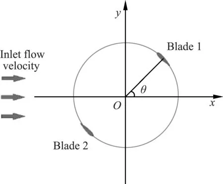
Fig.1 Coordinate system of vertical-axis marine current turbine
1.2 Computational domains and boundary conditions
The calculation domain of a two-dimensional marine current turbine is shown in Fig.2. The whole calculation model is divided into two sub-domains, namely, the rectangular outer domain and the circular rotation domain containing the blades of the VMCT.
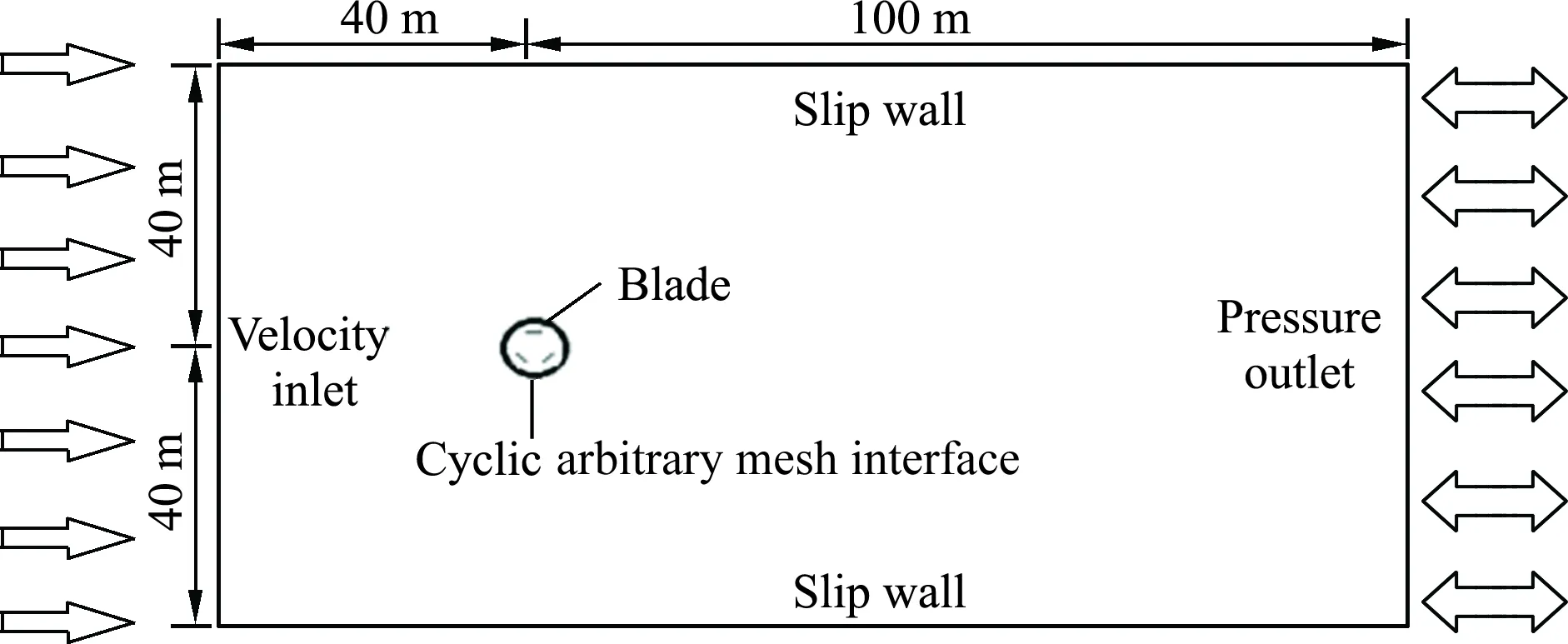
Fig.2 Calculation domains of vertical-axis marine current turbine
In the calculation example, the left-side boundary is set as the velocity inlet, and the velocity is constant. The right-side boundary is set as the pressure outlet and the relative pressure is 0. The upper and lower boundaries are set as the slip wall. The rotation domain and the rectangular domain are connected by a cyclic arbitrary mesh interface (AMI) boundary.
1.3 Solvers and turbulence models
The software used in this paper is OpenFOAM, an open-source CFD calculation software. The discrete method used is the finite volume method (FVM). On the basis of PISO-SIMPLE (PIMPLE) algorithm, the PimpleDyMFoam solver is selected to solve the transient solution of incompressible fluid Navier-Stokes equations[10].
The SSTk-ωmodel is selected as the turbulence model in this numerical simulation. The two-equation model combines the characteristics of thek-εandk-ωmodels to accurately simulate the sudden stall pheno-menon, and the calculation time is relatively small, which has been widely used in the research of MCTs[11-13].
2 Verification of numerical simula-tion methods

Tab.1 Related parameters of Strickland′s vertical-axis marine current turbine model
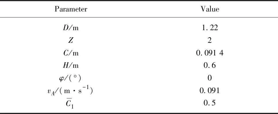
ParameterValueD/m1.22Z2C/m0.091 4H/m0.6φ/(°)0vA/(m·s-1)0.091C10.5
The experiment was carried out in a towing tank with a width of 5 m and a depth of 1.25 m. The curve of the tangential force coefficient and the normal force coefficient of a single blade at the tip speed ratio of 5.0 are given in reference [14].
The selected VMCT model is meshed, and the grid and time step are selected according to the nume-rical simulation of the vertical-axis turbine[14]. Structured grids with relatively good grid quality are selected and refined at each blade to improve the calculation accuracy. The model grids are shown in Fig. 3.
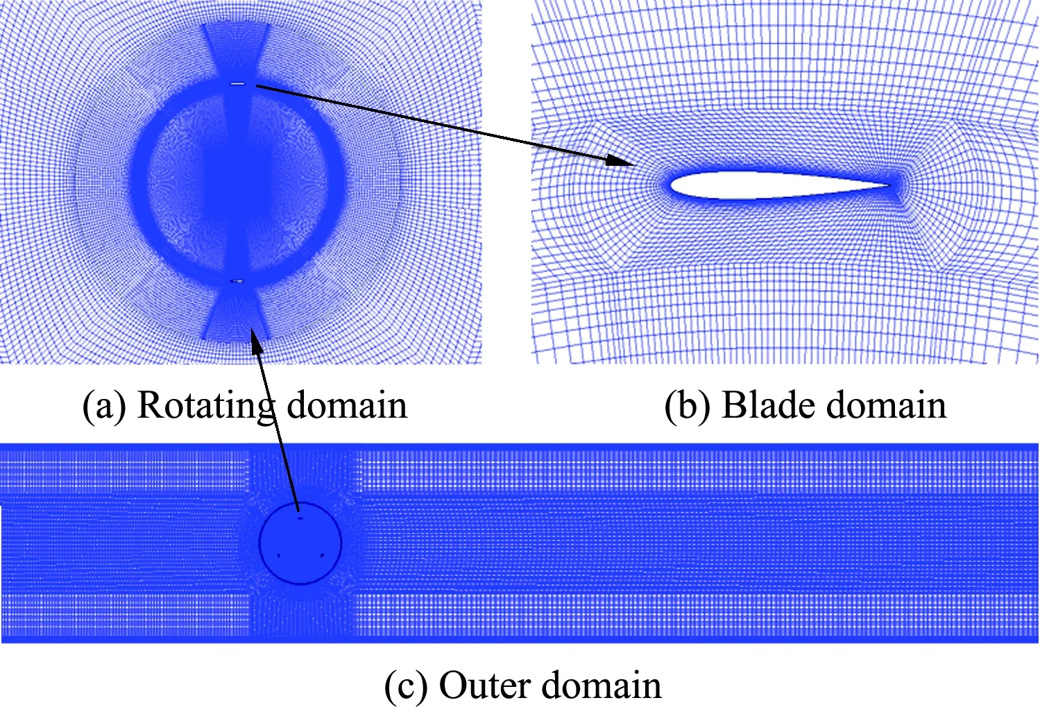
Fig.3 Mesh configuration
Fig.4 shows the comparison of the normal force coefficientCfnand the tangential force coefficientCftfor a single blade in the Strickland′s VMCT model at a tip speed ratio of 5.0. The trend of the curve between si-mulated and experimental values is approximately the same. The simulated value of normal force coefficient of the blade is in good agreement with the experimental value. The error mainly occurs between 180° and 360°, and the error of the blade tangential force coefficient mainly occurs near the 360° position angle. The simulation calculation method estimates the tangential force of the blade at a low level. Since this simulation method is a two-dimensional simulation without consi-dering the factors such as three-dimensional effects, experimental spokes, etc., there will inevitably be some errors between numerical simulation values and experimental values.
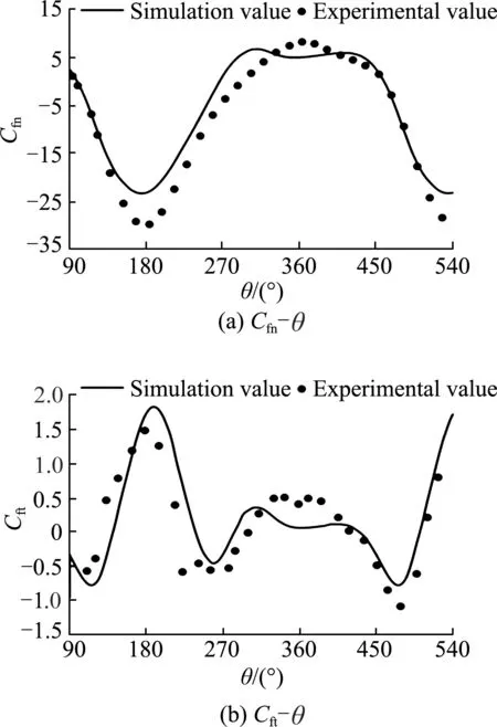
Fig.4 Comparison between simulation and experiment results
In summary, the difference between the simula-tion results and the experimental results is acceptable. It has been proved that the OpenFOAM software is feasible in predicting the hydrodynamic performances of VMCTs.
3 Influence of different parameters on vertical-axis marine current turbines
3.1 Influence analysis of the mesh
The mesh quality of the numerical model directly determines the accuracy of calculation and the length of simulation time. The fine mesh performs better in describing physical characteristics of the model, but the simulation time will also increase. Therefore, when selecting a mesh scheme, both time consumption and simulation accuracy should be considered. Taking a stand-alone VMCT as an example, three different levels of mesh models are analyzed and compared. The mesh specific information is given in Tab.2, whereZ1is the total mesh number;Z2is the rotation domain mesh number;tis the simulation time; Δhis the thickness of the first layer.
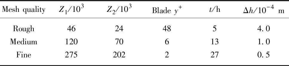
Tab.2 Detailed mesh information
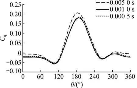
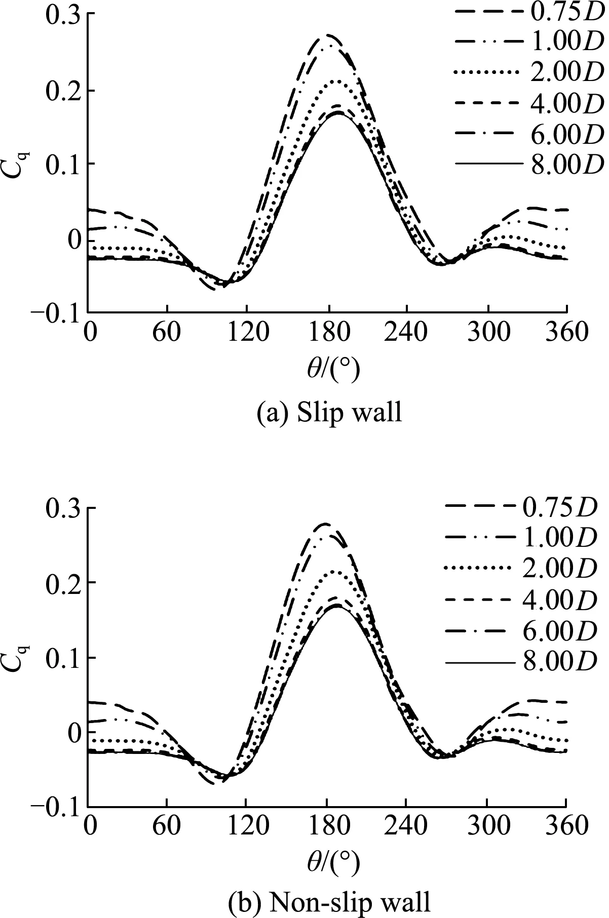
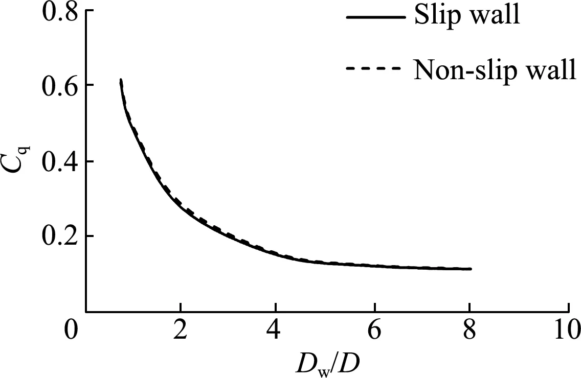
In Tab.2, the bladey+is the dimensionless coefficient of the first layer of the grid scale measured in the numerical simulation. The thickness of the first layer of grid on the wall is usually within a suitable range (5 (1) (2) (3) (4) whereρis fluid density;Lis a characteristic length;μis viscosity coefficient;Reis the Reynolds number;Cfis the friction coefficient;τwallis the wall tangential stress and Δhis the thickness of the first layer of grid on the wall. Fig.5 shows the variation trend of torque coeffi-cient of a stand-alone VMCT when the turbine rotates steadily under three different mesh schemes. It can be seen that the rough grid′sCqcurve differs greatly from the other two curves when it is between 150° and 210°; the difference between the medium and fine gridCqcurves is small, and the two curves are nearly completely coincident. Therefore, it can be judged that the medium-level grid basically meets the grid indepen-dence requirements while the simulation time of the fine-level grid is about 2.2 times of that of the medium-level grid. In order to save computing time, the medium-level grid is selected in the following nume-rical simulation. Fig.5 Variation trend of torque coefficient of stand-alone vertical-axis marine current turbine with phase angle for three different meshes In the transient simulation, 0.005 0 s, 0.001 0 s and 0.000 5 s are separately selected as time steps to study their influences on numerical simulation results. Fig.6 shows the torque coefficient of a single blade when the turbine rotates for one circle in three time steps. It implies that when the time steps are 0.001 0 s and 0.000 5 s, the torque curves almost completely coincide. In the calculation example of 0.005 0 s time step, the blade torque coefficient curve is generally higher than that of the other two curves. Therefore, it can be inferred that the time step is 0.001 0 s, which basically meets the independence requirement. At the same time, the simulation time step is smaller while the simulation time is longer. The running time step of the 0.000 5 s in this verification example is about twice that of the 0.001 0 s example. Therefore, consi-dering the finiteness and time consumption of calcula-tion resources, it is suggested that 0.001 0 s is selected as the time step for the example in the future. Fig.6 Torque coefficient variation tendency under different time steps At present, in the CFD study of VMCTs, there is neither uniform conclusion about the selection of wall types (slip wall, non-slip wall) nor reference distanceDwfrom the wall to the spindle center of the turbine in a two-dimensional simulation. Different standards are often recorded in different references. Therefore, in order to obtain a unified conclusion with reference value, the influence of wall type andDwvalue range on the hydrodynamic performances of VMCTs will be specifi-cally studied. Based on the above Strickland′s VMCT examples, the values ofDware 0.75D, 1.00D, 2.00D, 4.00D, 6.00D, and 8.00D, respectively (Dis the diameter of the turbine), and the wall types are slip wall and non-slip wall. The other parameters are unchanged (tip speed ratioλis 5.0), and the variation law of the torque coefficientCqand the turbine energy utilization coefficientCpof the turbine is compared and analyzed. The curve is shown in Fig.7. In the figure, it can be found that the turbine blades reach the maximum torque coefficient near the 180° position angle in each set of examples; the peak torque coefficient is significant and decreases with increasingDw. In addition, whenDwis less than 6.00D, the difference among the blade torque curves is larger and the blade torque coefficient increases as theDwvalue decreases; and whenDwis 6.00Dand 8.00D, the torque curve of the turbine blade almost completely coincides, which indicates that whenDwis not less than 6.00D, the sidewall boundary is far enough away from the turbine, that is, the effect of the sidewall on the hydrodynamic performance of the VMCT is negligible. Fig.7 Variation trend of torque coefficient of stand-alone vertical-axis marine current turbine Fig.8 Variation trend of the average energy efficiency coefficient of stand-alone vertical-axis marine current turbine From the perspective of the sidewall type, it can be seen that the core difference between the two types of sidewall surfaces (slip wall and non-slip wall) is that the slip wall surface only limits the normal velocity of the fluid to zero and has no limitation on the tangential velocity. The non-slip wall surface simultaneously limits the normal and tangential velocity of the fluid at the wall surface, that is, the flow velocity at the control wall surface is zero. The non-slipping wall surface is due to the presence of a viscous boundary layer at the wall surface, and there is no boundary layer in the slip wall example. It is worth noting that the thickness of the viscous boundary layer in this case is 0.1 m, which is negligible if compared with the calculation domain and the VMCT scale. It is relatively small, so the boundary layer has a small influence on the hydrodynamic performances of the VMCT. From the variation trend of average energy efficiency coefficient of the VMCT, it can also be found that the type of sidewall surface has almost no effect on the power characte-ristics of the VMCT. Therefore, in the transient numerical simulation of two-dimensional VMCTs, the sidewall surface can be arbitrarily selected from slip and non-slip types. Thus, the slip wall is selected as the sidewall surface type in the subsequent calculation examples. The definition of turbulence intensityIis shown in Equation (5). Equation (6) can be used to estimate the inlet turbulence intensityIin a fully developed pipeline flow. In the CFD simulation, it is usually ne-cessary to pre-estimateIat the inlet, that is, (5) I=0.16Re-1/8, (6) whereux(uy,uz) is the component of the inlet flow velocity in thex(y,z) direction. Tab.3 The average energy utilization coefficient varying with different turbulence intensities I/%0.10.51.05.010.0Cp0.4660.4640.4630.4620.460 Tab.3 implies that when the inlet turbulence intensity fluctuates in the range of 0.1%-10.0%, it has little effect on the average energy utilization coefficient of the VMCT. It is recommended that the inlet turbulence intensity be selected as 5.0% in the future numerical simu-lation of VMCTs. Based on open-source CFD computing software OpenFOAM, a numerical simula-tion method for vertical-axis marine current turbines is proposed and verified, which lays the foundation for subsequent optimization of algorithms based on open-source codes and more efficient calculations. Finally, the influence of different mesh schemes, time steps, sidewall type and inlet turbulence intensity of CFD numerical simulation is analyzed, and some empirical conclusions are drawn as follows: 1) Three different quality meshing schemes are proposed, and the optimal one is successfully obtained by comparison. 2) By comparing the calculation results of different time steps, the optimal one for the calculation of the double-blade vertical-axis marine current turbine is obtained. 3) Exploring the influence of the sidewall type on the hydrodynamic performance during the numerical simulation of the vertical-axis marine current turbines, it is concluded that the slip type and the non-slip type have less influence on the hydrodynamic performance of the two-dimensional case. 4) The influence of inlet turbulence intensity on the hydrodynamic performance of the turbine is small, and it is recommended that the turbulence intensity at the entrance is taken as 5.0%. The above conclusions will serve as a very valua-ble reference for the future two- and three-dimensional CFD numerical simulations of VMCTs. The authors would like to acknowledge the support of National Natural Science Foundation of China (Projects No. 11572094, No. 5171101175 and No. 51809083). In addition, the first author wants to acknowledge the CFD-China community for the fruitful OpenFOAM-related discussions. He also wants to thank his wife (Mrs. APP) for supporting his PhD work.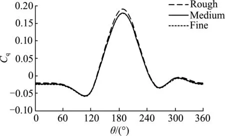
3.2 Influence analysis of the time step
3.3 Influence analysis of the wall type

3.4 Influence analysis of the turbulence intensity

4 Conclusions
5 Acknowledgement