Density limit disruption prediction using a long short-term memory network on EAST

Kai ZHANG(张凱),Dalong CHEN(陈大龙),Bihao GUO(郭笔豪),Junjie CHEN(陈俊杰) and Bingjia XIAO(肖炳甲)

1 Department of Engineering and Applied Physics,School of Physical Sciences,University of Science and Technology of China,Hefei 230026,People’s Republic of China

2 Institute of Plasma Physics,Chinese Academy of Sciences,Hefei 230031,People’s Republic of China

Abstract

Keywords:disruption prediction,tokamak,neural networks,flattop phase

1.Introduction

Disruptions of tokamak plasmas are important events in which the plasma energy is lost within a few milliseconds,and they present serious problems for the operation of tokamaks[1].During the disruption,the collapse of the plasma current and stored energy will create huge electromagnetic and thermal load on the device.In addition,a large number of runaway electrons will be generated during the disruption process,which may lead to the decomposition of some plasma-facing components[2].For the next generation of tokamaks like ITER(International Thermonuclear Experimental Reactor)or CFETR(China Fusion Engineering Test Reactor),the disruption mitigation system(DMS)is essential,which uses techniques such as massive gas[3]or shattered pellet injections[4]to suppress or eliminate potential disruptions.Moreover,highly accurate prediction of plasma disruption is the key to disruption mitigation[5].However,the physical mechanism of the disruption phenomenon is so complicated that it has not been clarified[6].Therefore,direct prediction of disruption in tokamaks using first principle theorems is a very difficult task.

Recently,with the development of machine learning techniques,the disruption prediction can possibly be achieved without actually understanding the detailed physics behind it.By training a model with a lot of pending parameters using past experimental data marked as disruptive or non-disruptive,the model may discover hidden physical laws from the data.Then,disruption in a new shot can be predicted[7].

Over the last 30 years,many machine learning methods have been developed for disruption prediction in tokamak devices,such as the JET[8],ASDEX-Upgrade[9],JT-60U[10],HL-2A[7]and J-TEXT[5].A real-time prediction system called APODIS using experimental data was developed in the JET,in which the support vector machine(SVM)algorithm is used[11-13].Prediction of β-limit disruptions in JT-60U was conducted using neural networks[14].Random forest models based on the experimental data of DIII-D,Alcator C-Mod and EAST have the advantage of interpreting and explaining the prediction[15-18].Manifold learning methods are also used to visualize and explore the highdimensional operational space[19-21].Convolutional neural networks are good at processing signals from multi-channels,and have been applied to disruption prediction in the HL-2A tokamak with great divergence[7].Furthermore,to extract spatiotemporal patterns from multimodal and high-dimensional sensory inputs,a specific architecture of a fusion recurrent neural network(FRNN),combining both recurrent and convolutional components has been applied[22].

A long short-term memory(LSTM)network should be highly recommended when faced with time series data,and LSTM combined with convolutional neural networks has been studied in recent years[7,22,23].But common recurrent neural architectures have the intrinsic difficulty in parallelizing their state computations[24],resulting in significant time costs.In this paper,LSTM is trained and tested on both flattop phase data and short time sequences,and the experiment results on short time sequences show a shorter training time and higher area under the receiver operation characteristic curve(AUC)compared to those on flattop phase data.However,in disruption prediction,the model performance in the flattop phase is significant.Since LSTM can handle variable-length sequences,the model trained on short time sequences is creatively applied to the entire flattop phase and the AUC is relatively high.The density limit disruption prediction is presented here.

The paper is organized as follows.Section 2 gives a short introduction to the advantage of using LSTM to perform predictions based on time series data.In section 3,we present the detailed setup and results with different approaches and their comparison of density limit disruption prediction on the EAST history data using LSTM.Finally,section 4 summarizes the conclusions.

2.Advantages of LSTM in disruption prediction using time series data

Firstly,we give a brief introduction to the process of disruption prediction using classical machine learning methods,like SVM.The data used for disruption prediction at a certain moment is a vector composed of the values of a plurality of diagnosis signals in the tokamak,which can be noted as a time slice.The vectors at different moments from disruptive shots are collected as positive samples and those from nondisruptive shots are collected as negative samples,which are used to train a discrimination model.In real-time prediction,each time a time slice is generated in the discharge process,the model is used to determine whether a potential disruption will occur.But making decisions with data from one moment can easily lead to misjudgment.According to the analysis using a self-organizing map(SOM)[25],the samples belonging to the ambiguous region are considered transition samples and they cannot be classified with sufficient confidence as either disrupted or non-disrupted samples[1].From a time perspective,this approach abandons time domain information.

The recurrent neural network(RNN)can generate the corresponding output after processing the input of each time step.Moreover,the output of the current time step in the RNN will be used as the input of the next time step[23].This special network structure can let the data at different time steps correlate with each other and,therefore,it saves the time domain information.So,the RNN provides an alternative way to process time series data for disruption prediction.The LSTM[26]network is a special type of RNN that overcomes the shortcomings of long-term dependence and the‘vanishing and exploding gradient’ problem[27]in original RNNs.Its central idea is a long-term memory cell which can maintain a state over time,and many gating units help to regulate the information flow into and out of the memory.Learning of LSTM can be carried out by a gradient descent method that is a combination of modified back propagation through time(BPTT)and modified real-time recurrent learning(RTRL)[28].A number of studies on time series and other sequential data that applied deep learning approaches indicated the advantageous properties of LSTM and other deep learning methods[29].

3.Density limit prediction on EAST using LSTM with different models

With labeled discharge data on EAST,the LSTM networks can be directly trained.However,the optimal prediction model may not be obtained in this way,which is shown in this section.Three kinds of models are trained and tested based on the EAST dataset:directly training and testing in the flattop phase,training and testing on short time sequences,and training on short time sequences while testing in the flattop phase.The performances of these models are compared.

3.1.Directly training and testing in the flattop phase

3.1.1.Dataset,label and model hyperparameters.In the present work,the dataset contains 300 density limit disruptive shots and 2921 non-disruptive shots that are randomly selected from the EAST past discharge shots No.60 000 to 73 000.For class balancing,150 disruptive shots and 150 non-disruptive shots are used as the training dataset,while 150 disruptive shots and 2771 non-disruptive shots are used as the testing dataset.Eleven kinds of diagnostic signals(plasma density,plasma current,internal inductance,radiation power at the core,radiation power at the edge,vertical plasma position,Mirnov probe,IC current,soft x-ray,poloidal beta,loop voltage)are used for the dataset[30].The plasma current flattop phase is intercepted as a dataset for each shot.Since different signals have different sampling rates and units,all the data are resampled at a rate of 1000 Hz and normalized between 0 and 1.

Shots have different discharge durations,so the dataset is unequal sequence data.Sequences of unequal length are padded with a specific number,which would help to train and test the model in a mini-batch way.The specific number would be masked during training and testing,thus having no effect on the trained model and test results.The shape of the training dataset is300×max_length×11,and that of the testing dataset is2921×max_length×11,where max_length is the length of the longest sequence in the dataset,300 is the number of discharge shots in the training dataset,2921 is the number of discharge shots in the testing dataset and 11 is the number of signals.The output sequence of the model is also filled to the longest sequence length of the input with the last moment output of the model.

The label is set to be the probability of disruption:0 means no disruption,and 1 means disruption has occurred.A value between 0 and 1 means that disruption is likely to occur,and a larger number indicates a higher possibility of disruption.The disruptive shot is divided into two phases:the safe phase and the disruptive phase.The length of the disruptive phase is empirically set to 400 ms,and the disruptive phase is the period before disruption occurs.The remaining period is the safe phase.Such dividing of phases can also be found in[17,31,32].The label in the safe phase is set to 0,and the label in the disruptive phase is obtained by sampling the sigmoid function(equation(1))at[−5,5],of which the value is between 0 and 1.This labeling is also used in previous work by Cannas et al[33].For nondisruptive shots,all the labels are set to 0.Examples of the label setup are shown in figure 1.

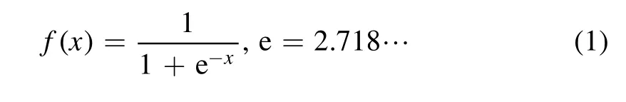
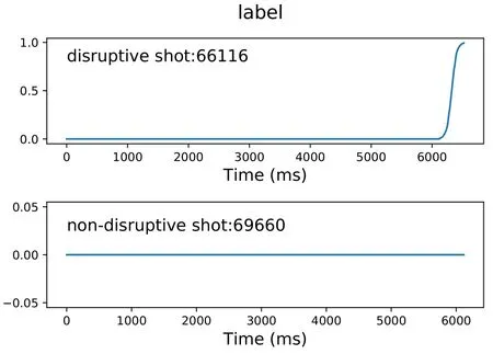
Figure 1.The label setup for disruptive shot 66116 and nondisruptive shot 69660.

Some discharges are randomly extracted from the training dataset as a validation dataset to determine hyperparameters.The model consists of two layers of LSTM networks,with the LSTM cell numbers of the first and second layers set to 200 and 1.The optimizer is the Adam algorithm[34],and the loss function is the mean square error(MSE).The training suspension condition is that the loss of the training dataset no longer drops.

3.1.2.Model testing and evaluation.When the time slice in the testing dataset is entered into the model,the model will predict the probability of disruption.The disruption alarm threshold is preset by us.If the model outputs of a discharge exceed the threshold,it is determined as a disruptive shot,and if the model outputs of a discharge are all lower than the threshold,it is determined to be a non-disruptive shot.

The binary classification problem evaluation index is the sensitivitySnand the specificitySp:

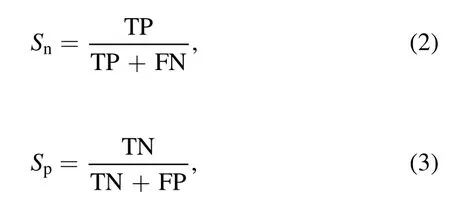
whereTP refers to a disruptive shot that is correctly identified as a disruptive shot,FN refers to a disruptive shot that is misidentified as a non-disruptive shot,TN refers to a nondisruptive shot that is correctly identified as a non-disruptive shot andFP refers to a non-disruptive shot that is misidentified as a disruptive shot.TP,FN,TN and FP are determined by considering global shots.In other words,the assessment of the predictor is carried out on a shot-by-shot basis,rather than slice-by-slice.Examples ofTP,FN,TN,FP predictions are shown in figure 2.

In practice,the higher the sensitivity and specificity,the better the prediction model.Raising the threshold,more discharge shots are identified as non-disruptive shots:Sprises andSnfalls.Lowering the threshold,more discharge shots are identified as disruptive shots:Snrises andSpdrops.Here,the best threshold is estimated by maximizing the Youden index[35]:

The AUC value[36],which is the area under the receiver operation characteristic(ROC)curve[37],can be used to evaluate the quality of different models.In a trained model,each threshold corresponds to a set of pairs(Sp,Sn).When varying the threshold,many pairs are obtained.On a ROC curve,the horizontal axis represents the false positive rate(1−Sp),and the vertical axis represents the true positive rateS.nThese pairs are drawn and connected to obtain the ROC curve.When the AUC is 0.5,the model does not have any classification ability.Overall,the closer the AUC is to 1,the better the classification performance of the model.

Another performance feature of the model is the warning time.When the predicted disruption probability of the model exceeds the threshold,an alarm should be triggered.The warning time is defined as:

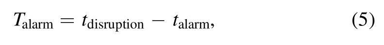
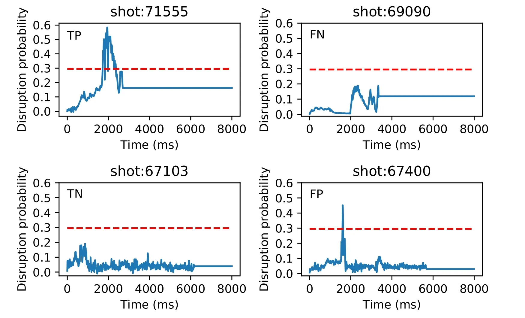
Figure 2.Examples of TP,FN,TN and FP predictions.The red dotted line represents the threshold=0.295,and the blue solid line represents the predicted disruption probability,which is the output of the model.Shots 71555 and 69090 are disruptive shots.Shots 67103 and 67400 are non-disruptive shots.

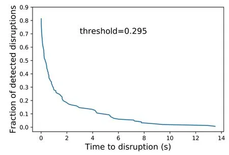
Figure 3.The fraction of detected disruptions as a function of the time to disruption for an ‘optimal’ threshold value.

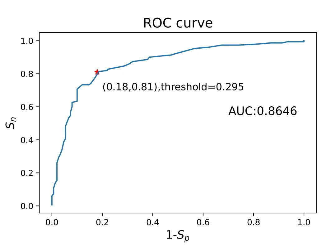
Figure 4.The ROC curve of a model with AUC=0.8646,in which the best threshold is estimated by maximizing the Youden index and the corresponding point is marked with a red star.The model is both trained and tested in the flattop phase.

wheretdisruptionis the time when the disruption really occurs,andtalarmis the time when the disruption probability of the model output exceeds the threshold.In practice,the DMS needs some time to take action.Only when the warning time is longer than the cut-off time can the corresponding disruptive shot be considered as correctly predicted.Here,the cut-off time is set to 10 ms,and a disruptive shot with a warning time less than 10 ms is considered as FN.Furthermore,the relation between warning time and fractions of detected disruptions is plotted in figure 3,in which late alarms are also discarded.

The 3221 discharges are randomly divided into a training dataset(containing 300 shots)and testing dataset(containing 2921 shots),and a trained model and the corresponding test results can be obtained.To reflect the general law,the operation is repeated ten times.Therefore,ten models with the same hyperparameters are trained on different datasets.The highest AUC of the ten models is 0.8646,and the corresponding ROC curve is shown in figure 4.Detailed AUC values of these ten models can be found in the second column of table 1.

Table 1.AUC values of the models.

3.2.Disruption prediction on short time sequences

In this section,the same 3221 shots are used as in section 3.1,and the last 1000 ms of the flattop phase of each shot is intercepted as the model input.The shape of the training dataset is300×1000×11,and the shape of the testing dataset is2921×1000×11.Other parameters,including label choice and model hyperparameters,are the same as in section 3.1.1.The training dataset and testing dataset are randomly selected.This experiment is repeated ten times,and ten models and the corresponding test results are obtained.

Similar to section 3.1.2,the AUC is used as the model evaluation index.The third column of table 1 shows that the highest AUC reached among the ten trained models is 0.9379.The best point is chosen on the ROC curve of the best model by maximizing the Youden index,and the corresponding threshold is 0.55,shown in figure 5.Examples of TP,FN,TN and FP are shown in figure 6.With the threshold being 0.55,the warning time is evaluated in figure 7.

The computer configuration used for the training model is Intel i7-7700 3.6 GHz,16 GB RAM.With the same model structure and hyperparameter settings,training the model with flattop data takes 6900 s per epoch,however,training the model with short time sequences only needs 36 s per epoch(in one epoch,all training data are used once).This is because the RNN represented by LSTM is sensitive to the length of the sequence,and a longer time series needs more training time.

Comparing the results of sections 3.1 and 3.2,it is found that while training the model directly from the flattop phase data,and using the model to test in the flattop phase,the highest AUC can reach 0.8646.While training the model with short time sequences and testing on short time sequences,the AUC can easily reach above 0.9,and the highest AUC can reach 0.9379.This may be due to the fact that,for disruptive shots,only a small part of the time period contains disruption precursors.A too-long time series can easily cause disruption precursors to be drowned in a large amount of data.Short time sequences from the flattop phase are intercepted to train the model,which is equivalent to amplifying this disruption precursor in the data.

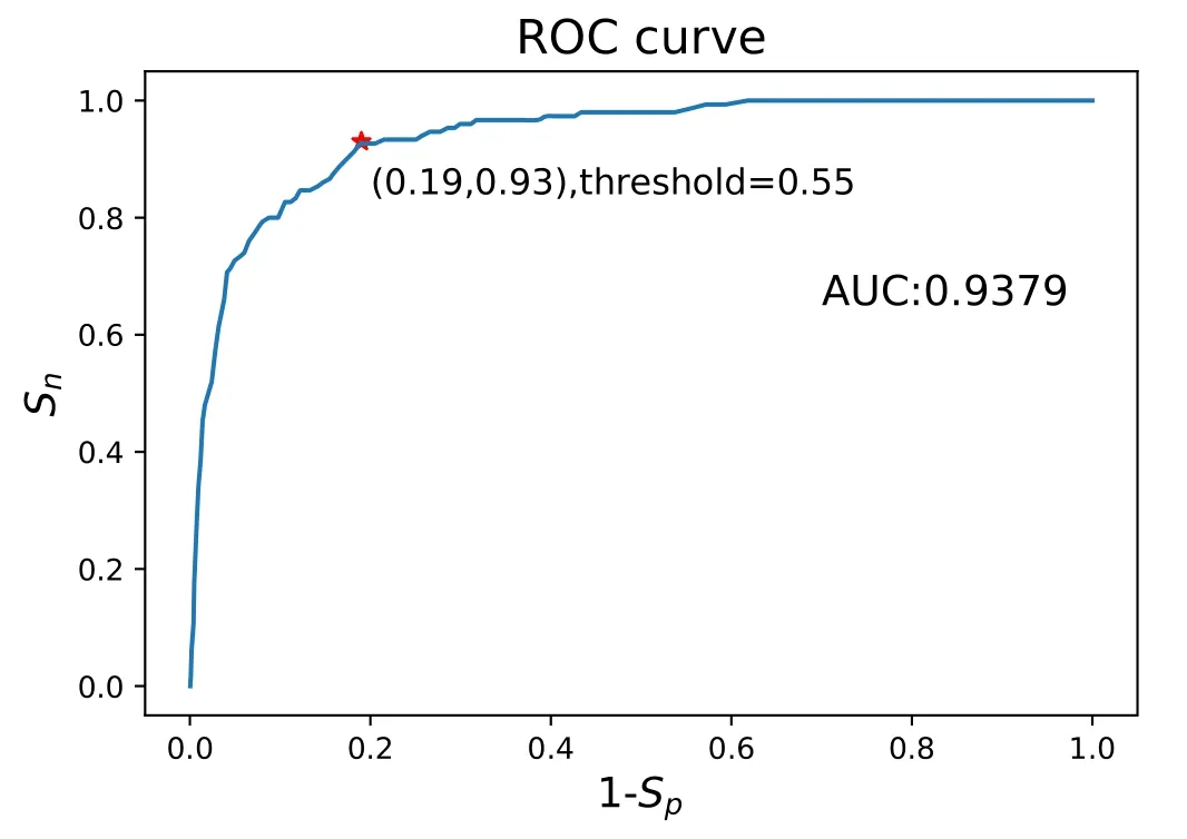
Figure 5.The ROC curve of a model with AUC=0.9379,in which the best threshold is estimated by maximizing the Youden index and the corresponding point is marked with a red star.The model is both trained and tested on short sequences.

3.3.Model migration

In section 3.2,the model is trained on short time sequences and tested on short time sequences,achieving a higher AUC compared with the model in section 3.1.However,it has no practical value for real-time disruption prediction since we never know when a disruption occurs and when it is 1000 ms before the disruption.An ideal disruption prediction model should be able to output predicted possibilities in real time starting from the beginning of the plasma discharge.Currently,this goal is difficult to achieve on EAST.Here,the compromise,which is to start with the plasma current reaching the flattop phase,is adopted in the present work.

Note that the input of one trained LSTM model can be a sequence of data of arbitrary length.Therefore,the models trained in section 3.2 can be directly used to predict the possibility of a discharge on a whole flattop.The corresponding AUC results are shown in the last column of table 1.The highest AUC achieved is 0.9189,which is also obtained by the best model in section 3.2,and it is also higher than all the AUC values of the models in section 3.1.

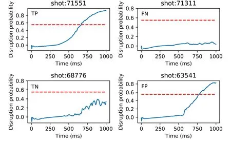
Figure 6.Examples of TP,FN,TN and FP predictions.The red dotted line represents the threshold=0.55,and the blue solid line represents the predicted disruption probability which is the output of the model.Shots 71551 and 71311 are disruptive shots.Shots 68776 and 63541 are non-disruptive shots.

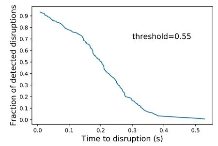
Figure 7.The fraction of detected disruptions as a function of the time to disruption for an ‘optimal’ threshold value.

The best point on the ROC curve of the best model is chosen by maximizing the Youden index,and the corresponding threshold is 0.89,shown in figure 8.Examples of TP,FN,TN and FP are shown in figure 9.With the threshold being 0.89,the warning time is evaluated in figure 10.

Figure 8.The ROC curve of a model with AUC=0.9189,in which the best threshold is estimated by maximizing the Youden index and the corresponding point is marked with a red star.The model is trained on short sequences and tested on flattop phases.

When the model was trained on data from the last 1000 ms of the flattop phase and tested in the same period,the AUC of the model can reach 0.9379.When the models trained on short time sequences are applied to the flattop phase data for testing,it is found that the AUCs are better than those of the models trained in the entire flattop phase.It is worth mentioning that the model trained on data from the last 1000 ms of the flattop phase had never seen data from the beginning part of the flattop phase,but it can still achieve a good performance throughout the entire flattop phase.This shows that LSTM networks can effectively extract disruption precursor features from short time sequences.

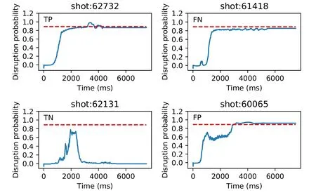
Figure 9.Examples of TP,FN,TN and FP predictions.The red dotted line represents the threshold=0.89,and the blue solid line represents the predicted disruption probability,which is the output of the model.Shots 62732 and 61418 are disruptive shots.Shots 62131 and 60065 are non-disruptive shots.

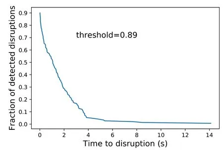
Figure 10.The fraction of detected disruptions as a function of the time to disruption for an ‘optimal’ threshold value.

4.Conclusions

Although the LSTM network has the advantages of prediction with series data,it is found that using the entire flattop data to train the model takes a long time and it is not ideal.Alternatively,using only short time sequences to train the model takes a very short time,and the model still has good performance when applied to the entire flattop phase.Such a model training strategy improves LSTM performance in the flattop phase and shortens training time.

The problem of early warning in the experiments is very serious.In figures 3 and 10,more than 20% and 40% of the disruptive shots trigger an alarm more than 1 s in advance,respectively.Such early warnings would imply missing a lot of experimental time in these discharges.Vega et al[38]developed a disruption time predictor,which would be essential to avoid the shutdown of discharges several seconds in advance.Implementing a disruption time predictor will be future work.

Acknowledgments

The work is supported by the National Magnetic Confinement Fusion Energy R&D Program of China(2018YFE0304100 and 2018YFE0302100),Anhui Provincial Natural Science Foundation(1808085MA25).

The authors wish to thank all the members at the Institute of Plasma Physics,Chinese Academy of Sciences for providing past experimental data on EAST.