Effect of non-condensable gas on a collapsing cavitation bubble near solid wall investigated by multicomponent thermal MRT-LBM∗

Yu Yang(杨雨), Ming-Lei Shan(单鸣雷), Qing-Bang Han(韩庆邦), and Xue-Fen Kan(阚雪芬)

1Jiangsu Key Laboratory of Power Transmission and Distribution Equipment Technology,Hohai University,Changzhou 213022,China

2College of Computer and Information,Hohai University,Nanjing 210000,China

Keywords: multicomponent,cavitation bubble,non-condensable gas,lattice Boltzmann method

1. Introduction

Cavitation is ubiquitous in the natural and industrial fields. A cavitation bubble collapsing near a solid wall will lead the extreme conditions to form locally,such as high pressure, temperature and velocity.[1]Owing to these cavitation properties,research on the potential of cavitation exploitation is currently an interesting topic. Some optimized applications of cavitation have been established, such as cavitation degradation,cavitation sterilization,and lab-on-chip.[2–4]However,cavitation treatment is difficult to optimize because the mechanisms of the cavitation phenomenon are not completely illustrated in the presently reviewed literature.

Many numerical simulation methods have been suggested to investigate the collapsing cavitation bubbles because experiments are difficult to conduct and are deficient in capturing the internal mechanism of cavitation bubbles. Computational fluid dynamics (CFD) methods have been successfully employed for the simulation of multiphase flow.[5]However,they require complex interface-tracking or interface-capturing technology, and interactions among the constituent molecules on a microscopic scale cannot be considered. In contrast to conventional CFD methods,the lattice Boltzmann method(LBM)based on the microscopic nature and mesoscopic characteristics performs well in the numerical simulations of complex gas-liquid phase change. The main advantages, such as clear physical background,perfect parallel computing scheme, linear convection term, and extraordinary capability of dealing with complex boundaries, distinguish the LBM from other numerical methodologies. The Shan–Chen[6]pseudopotential method stands out in comparison with other multiphase lattice Boltzmann (LB) models because of its simple implementation and automatic separation of phases or components without interface-tracking or interface-capturing.

In the last two decades, many efforts have been made to apply the pseudopotential LBM to investigating the phase change and heat transfer phenomena,such as cavitation,evaporation, and boiling.[7–9]Several models have been established by introducing thermal equations into LB multiphase models.[10–12]Generally, thermal LB models are divided into three categories: the multispeed approach,[13]the doubledistribution-function (DDF) approach,[14,15]and the hybrid approach.[16,17]Among them,the pseudopotential DDF model proposed by Zhang and Chen has been widely used in the simulation of multiphase flow with phase change.[18]Later,Gong and Chen improved the thermal LBM by adding a new form of the source term to the temperature distribution function,thus reducing the spurious currents.[19]Meanwhile,multicomponent (MCP) LB models are being developed rapidly.[20,21]Bao and Schaefer considerably improved the multicomponent multiphase model,but thermal effects have not yet been incorporated into this model.[22]Qin et al. studied the heat transfer of multicomponents by using a single temperature evolution equation.[23]Ikeda et al. proposed a thermal immiscible multicomponent LB model.[24]In their model, each component employs the respective temperature equation, and then the temperature is coupled at each node by using the densityweighted combination. Later, one addressed many aspects of the multicomponent thermal model, such as the large density ratio, spurious current and numerical instability.[25–28]This advances the LBM closer to the realistic physical phenomena in simulating multicomponent multiphase flow.

Based on single-component DDF LBM, Yang et al.[29]used the improved thermal multiple-relaxation-time (MRT)-LBM model to simulate a collapsing cavitation bubble and discussed the effects of the position offset parameter and pressure difference on the maximum temperature of the bubble. However, cavitation bubble contains vapor and non-condensable gas in real physical phenomena. Some studies indicate that experiments with a small non-condensable gas concentration inside the bubble show its strong influence on the dynamics and thermodynamics of the bubble.[30,31]However, the internal influence of the non-condensable gas on the collapsing cavitation bubble cannot be explained at a microscopic level.Therefore,it is of great significance to study the effect of noncondensable gas inside bubble on the bubble collapsing near a solid wall by using numerical methods. To the best of the author’s knowledge, little researches have been reported on the dynamic and thermodynamic behaviors of multicomponent cavitation bubble by using LBM in the literature.

In the present work,a developed multicomponent thermal MRT-LBM is presented to numerically study the collapsing cavitation bubble. The rest of this paper is organized as follows. The basis numerical model is presented in Section 2. In Section 3 the model verification and computation domain are described. In Section 4 the effect of the non-condensable gas inside bubble on a collapsing bubble near a wall is illustrated.In Section 5 the conclusions and discussion are presented.

2. Multicomponent lattice Boltzmann methods

2.1. Pseudopotential MRT-LBM

The multicomponent evolution equation of the density distribution function with the MRT collision operator can be given by[32,33]

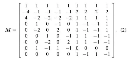
and the diagonal matrix is written as

The macroscopic Naiver–Stokes(NS)equation can be derived from Eq. (1). The mass and momentum equations of each component are as follows:[35,36]

where ασis the volume fraction satisfying α1+α2=1. The range of α1and α2are both 0–1. According to Eq.(4),we can obtain the continuity equation for the mixture

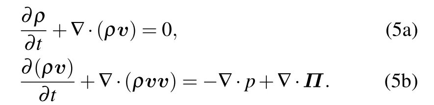
For the incompressible or slightly compressible fluids,the viscous stress tensor is

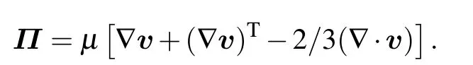
The average dynamic viscosityµ =α1µ1+α2µ2.

Using the transformation matrix, equation (1) can be transformed into

The multicomponent moment space can be obtained from the following expression:

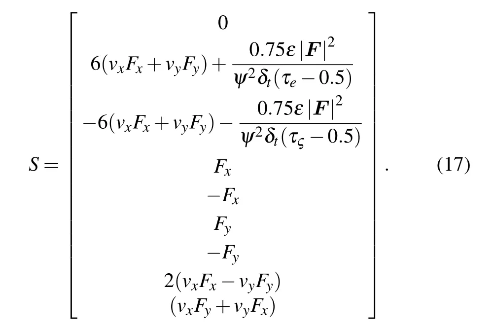
mσ = M fσ=Mij,σfj,σ=(ρσ,eσ,ςσ,jx,σ,qx,σ,jy,σ,qy,σ,pxx,σ,pxy,σ)T, (8)

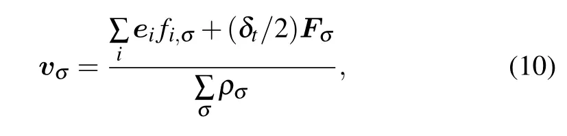
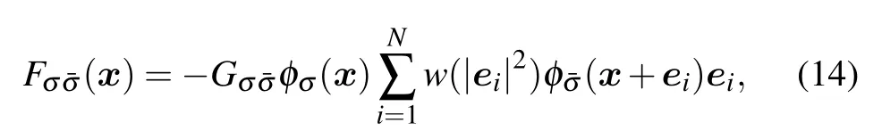
where Fσ=(Fx,σ,Fy,σ) refers to the total force of the fluid–fluid interaction acting on the system. Both the intramolecular force and intermolecular force exist in the multicomponent system. The intramolecule force can be expressed as

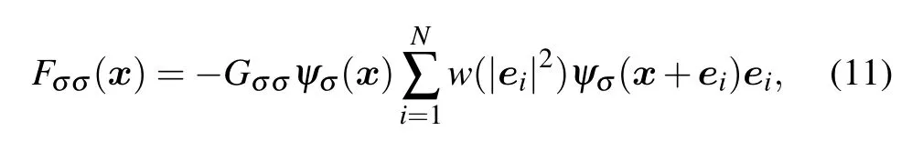
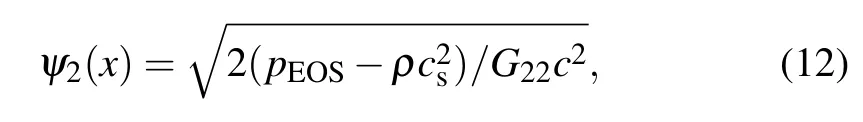
where Gσσis the intramolecule interaction strength. In this study,the subscripts σ =1 and σ =2 represent the gas phase and liquid phase,respectively. The gas is regarded as the ideal fluid and thus G11=0. The liquid is the non-ideal fluid. The weight wi=1/3 for |ei|2=1 and the weight wi=1/12 for|ei|2=2 on D2Q9 lattice for the nearest-neighbor interactions.The interaction potential ψ2(x)is adopted to mimic the interaction force of liquid,which is given by[37]

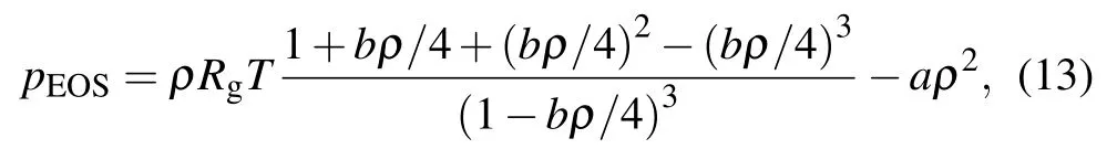
where a=0.4963(RTc)2/pc, b=0.1873RTc/pc, and Rg=1 is the gas constant,with Tcbeing the critical temperature,and the critical pressure.The constants a=1 and b=4 are used in the present study. For the gas component,the pseudopotential is equal to its density. The intermolecule force is determined by[39]

The improved forcing scheme proposed by Li et al.[40]is adopted in the present model. An adjustable coefficient ε as shown in Eq. (17) is employed to adjust the pseudopotential LB model to achieve good thermodynamic consistency and improve the mechanical stability of the model. In this work,based on the investigation of the thermodynamic consistency,ε is set to be 1.86 for the liquid component. For the gas component,just set ε =0.

2.2. Thermal MRT-LBM

The temperature in an EOS can be derived by solving the target temperature equation[41]

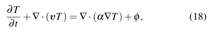
where α =k/ρcvis the thermal diffusivity, k is the thermal conductivity, ρ is the macroscopic density, cvis the specific heat at a constant volume,and φ is the source term of the temperature.

In order to solve the target temperature equation, an improved thermal LB model based on the MRT collision operator is used in this model.[42]To simulate the temperature evolution process of gas–liquid two-phase component, the temperature distribution function of the σ-th component is given by

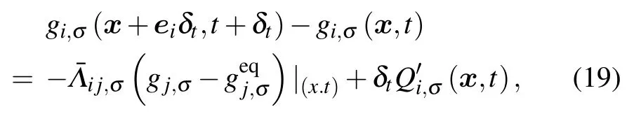
In numerical implementations, ∂tφσ≈ [φσ(t) −φσ(t −δt)]/δt.

Unless otherwise specified,the unit adopted in this paper is the lattice unit of the LBM.The basic units of length,time,and mass are lu (lattice unit), ts (time step), and mu (mass unit),respectively. Thus,the units of density,pressure,velocity, and viscosity are expressed as mu/lu3, mu/(ts2·lu), lu/ts,and lu2/ts,respectively.

3. Verification of spherical cavitation bubble

3.1. Validation of Laplace law

For the cavitation bubble case, Laplace law shows that the pressure difference between both sides of the bubble is inversely proportional to the bubble radius, which can be expressed as

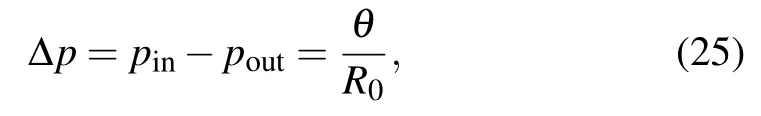
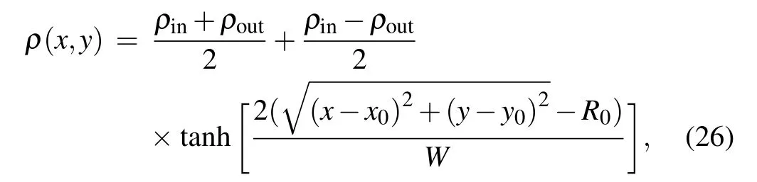
where pinand poutare the pressure inside and outside the bubble,respectively,R0is the initial bubble radius and θ is the surface tension. An approximately pure gas bubble surrounded by liquid is placed in the center of the periodic domain in a gravity-free field. The density field is initialized into[43]where ρinand ρoutare the density inside and outside the bubble,respectively. (x0,y0)is the center position of the domain.The width of the phase interface W =5. The hyperbolic tangent function tanh(x)=(e2x−1)/(e2x+1). The computational domain is a 201×201 lattice system. Initially, the density of gas(liquid)is 0.003(0.00001)and 0.000001(0.42)inside and outside the bubble, respectively. The initial radius R0is set to be 20, 25, 30, 35, and 40. The results at the different reduced temperatures are shown in Fig.1. The linear relation between the pressure difference ∆p and 1/R0can be clearly observed,indicating that the simulation results accord well with those from the Laplace law.

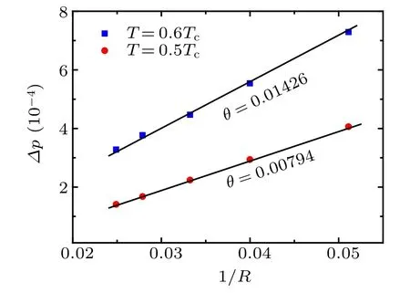
Fig.1. Plots of ∆p versus 1/R0,showing validation of Laplace law.

3.2. Comparison between simulation results from RP equation and Rayleigh bubble collapse

The Rayleigh–Plesset (RP) equation can be used to describe the dynamical behavior of cavitation bubble growth and collapse. In order to verify the consistency of the LBM simulation results of the cavitation bubble collapse with the numerical solution of the RP equation, a model of a spherical cavitation bubble with radius R(t)in an infinite liquid field is established as shown in Fig.2. The bubble is assumed to be a mixture of non-condensable gas and vapor. The liquid temperature T∞is considered to be homogeneous. The pressure inside the bubble pb(t)includes the vapor pressure pvand the partial pressure of non-condensable gas pg. The pressure far from the bubble is p∞(t),which is regarded as a known input parameter to control the growth and collapse of the bubble.

Under the above assumptions,the RP equation is written as[1]

According to the Meyer equation

the relationship between γ and cvcan be obtained by combining Eqs.(28)and(29)as follows:

Fig.2. A spherical cavitation bubble in infinite liquid field.

The specific heat at constant volume is chosen to be cv=3 in this paper. Thus, the adiabatic coefficient is γ =1.3. For this calculation comparing the numerical and RP equation solutions,the solution of the RP equation is obtained by substituting the corresponding LBM parameters into Eq.(27). The initial densities of the system are the same as those in Subsection 3.1,and the surface tension is chosen to be θ =0.01426.The pressure difference ∆p= p∞−pb=0.0325 is obtained by artificially setting a density difference to trigger bubble collapse. Meantime, the single-component (SCP) model is added as the control group,that is,the bubble containing noncondensable gas is replaced by the vapor bubble in the computation domain. The initial densities of vapor and liquid are ρv=0.00306 and ρl=0.406 at 0.6Tc, respectively. The numerical simulation domain is 201×201. Periodic boundary conditions are adopted in all directions. The instantaneous radius is normalized by the initial radius R0, and the time is non-dimensionalized by the total simulation time step.

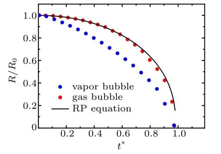
Fig.3.Comparison among radius evolutions with time of collapsing bubble,obtained from three calculation methods.

Figure 3 shows that the MRT-LBM simulation results accord with the results from the law of Rayleigh bubble collapse. It is verified that the multicomponent LBM method can simulate the dynamic behavior of a cavitation bubble containing non-condensable gas. Additionally, the slope of the blue dot curve is higher than that of the red dot curve. It is illustrated that the collapse velocity of the bubble containing noncondensable gas is lower than that of the vapor bubble. Thus,the non-condensable gas weakens the collapse velocity of a cavitation bubble.

3.3. Validation of adiabatic law

In this section,it is shown that the thermal model can be used to simulate the temperature evolution of the collapsing bubble. Because the collapse time of the cavitation bubble is nearly instantaneous (on the order of microseconds), it is generally considered that the process from cavitation bubble shrinkage to complete collapse is adiabatic. The formula for calculating the maximum temperature at the instant of bubble collapse under the adiabatic law is given by[1]

where T∞is the ambient temperature in the liquid, R0is the initial bubble radius, and γ =1.3 is a constant representing the adiabatic coefficient of the ideal gas. The pressure difference ∆p=0.0325. The evolution process of the temperature field of a collapsing cavitation bubble in an infinite domain and the corresponding central temperature curve of the bubble are shown in Fig.4. The instantaneous temperature is normalized by the critical temperature Tc, and the time is nondimensionalized by the total simulation time step.

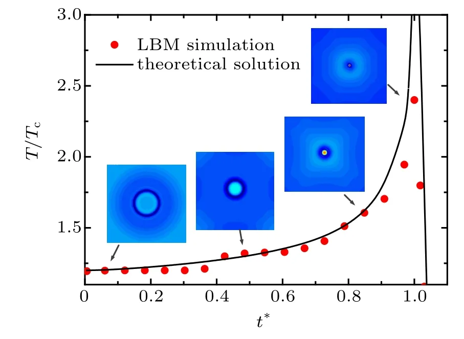
Fig.4. Plot of T/Tc versus t∗,showing verification of adiabatic law.

It is worth mentioning that the maximum temperature of the bubble collapse can theoretically reach infinity. This is because the theoretical model usually neglects the effects of heat dissipation and viscous dissipation.However,such a high temperature cannot be reached due to dissipation and other factors in the experiment or the LBM simulation.These methods have a common trend of temperature increase. As shown in Fig.4,the trend of the LBM numerical simulation is consistent with that of the theoretical solution.

4. Effect of non-condensable gas in bubble on collapsing bubble near solid wall

Due to the complexity and unpredictable nature of cavitation, the progress of revealing its thermal behavior and consequences need to be analyzed by multicomponent thermal LBM.The thermal effect of the collapsing bubble can be described more accurately by considering the action of noncondensable gas. In order to study the thermodynamic mechanism of the bubble containing non-condensable gas,a numerical model of cavitation bubble near a solid wall is established.

4.1. Computational model

The computational simulation domain of the cavitation bubble collapse near a solid wall is set to be a 201×201 lattice as shown in Fig.5, where R0is the initial radius of the bubble,b is the distance from the bubble center to the solid wall,and the offset parameter λ =b/R0is defined as the standoff distance between the bubble center and the lower wall. The bottom boundary is set to be a rigid plane boundary with a bounce-back boundary condition.[34]Periodic boundary conditions are adopted in the left and right direction.Additionally,an anti-bounce-back approach is adopted at the top of the computational domain by the open boundary.

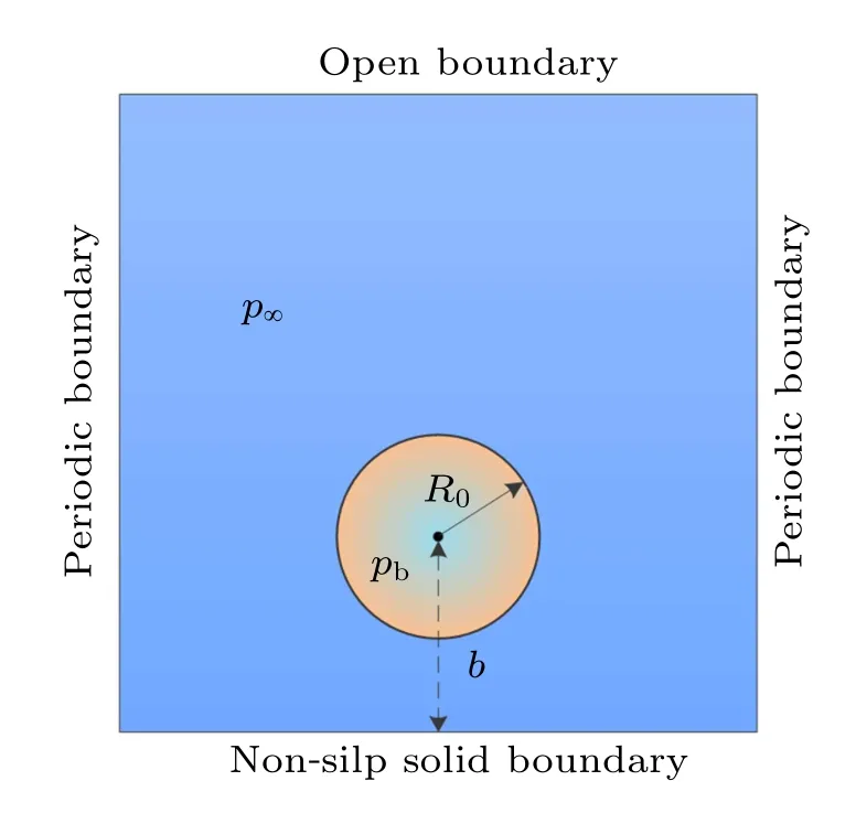
Fig.5. Computational domain.

The initial bubble volume is constant, and thus the volume fraction of the gas and vapor are important adjustable parameters. Three cases of the initial volume fractions of the non-condensable gas and vapor in the bubble are given in Table 1. They are used to investigate the different morphologies and thermodynamics of collapsing under different volume ratios of the gas to the vapor. In this study, only the noncondensable gas and vapor volume in the bubble are considered to be variable,and the remaining initial conditions are invariant. In the simulation,the initial radius of the bubble is determined to be R0=40.The initial liquid density is ρl=0.406 at 0.6Tc. The pressure difference ∆p= p∞−pb=0.0358. In our present work,[44,45]the obvious secondary collapse can be observed when the offset parameter λ =1.4 of the SCP bubble collapses near the wall. Therefore,the offset parameter is chosen to be λ =1.4 as the reference parameter in this MCP model.

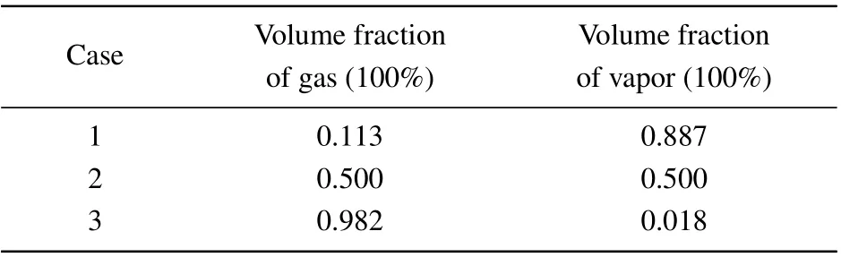
Table 1. Initial volume fraction of non-condensable gas and vapor in bubble.

4.2. Cavitation bubble collapse near solid wall

The results are presented, with the pressure field on the left and the temperature on the right,and due to the symmetry of the cavitation bubbles in Figs. 6–8, emphasis is placed on the temperature field.

The cavitation bubble in case 1 can be considered as an almost vapor-filled bubble. As shown in Figs. 6(a)–6(c), the bubble deforms from a spherical bubble to an elongated bubble in a direction perpendicular to the solid wall. The radial liquid flow is retarded because of the solid wall, and a region with reduced pressure/temperature is formed near the solid wall. A conical high-pressure region is formed above the bubble due to the rebound of the liquid and the relatively high liquid velocity. The temperature inside the bubble is observed to increase gradually. The bubble collects the energy from the surrounding liquid,resulting in a lower temperature at the interface between the bubble and liquid. A micro-jet flow is formed on the top of the bubble as shown in Fig.6(d). The first collapse occurs as shown in Fig.6(e), and the jet directs toward the boundary and hits the lower bubble wall. Hence,the bubble becomes toroidal. Owing to the driving effect of the jet,the toroidal bubble rapidly collapses as shown in Fig.6(f),which is called the second collapse. Because the time interval between the first collapse and the second collapse is extremely short, the high-temperature and high-pressure shockwaves created by the second collapse hit the wall almost simultaneously with the first collapse as shown in Figs.6(g)and 6(h). The waves damage the wall and form a hotspot as shown in Figs.6(i)and 6(j). Then,the residual wave diffuses into the surrounding liquid until it vanishes.

Figure 7 shows the simulation results for case 2. The evolution processes of the pressure and temperature fields before the first collapse are displayed in Figs. 7(a)–7(c) and are similar to those in Figs. 6(a)–6(e). After the first collapse (Figs. 7(d) and 7(e)), the high-temperature and highpressure shockwaves hit the solid wall perpendicularly. The second collapse is shown in Fig.7(f). The visible bubble wall disappears completely, and a high-pressure and hightemperature toroidal bubble is formed. Meanwhile, owing to the water hammer effect, a clear high-pressure and hightemperature domain is formed on the solid wall. The central temperature of the toroidal bubble is reduced. As shown in Fig.7(g), when the waves created by the high-pressure and high-temperature toroidal bubble propagate outward, another low-pressure toroidal region is formed in situ due to the rebound effect of the liquid.

As shown in Figs. 7(g)–7(j), the pressure waves created by the second collapse are converged and superimposed on the symmetry axis,forming a high-pressure region,which immediately diffuses upward and downward. The temperature waves first diffuse the radiation waves from the collapse points to the surroundings. Then, the high-temperature waves reach the solid wall together with the high-pressure waves. Therefore,a hotspot region is formed on the wall,which intensifies the cavitation erosion. According to the second law of thermodynamics, energy can be transferred spontaneously from a high-temperature region to a low-temperature region. The high-temperature waves created by the bubble radiate in all directions and eventually vanish. The lower temperature region of the toroidal bubble gradually reaches the surrounding liquid temperature.

Figure 8 shows the evolutions of pressure and temperature in case 3. The bubble is considered to be a non-condensable gas-filled bubble with little vapor. The evolution processes in Figs.8(a)–8(f)before the second collapse are similar to those in Figs. 7(a)–7(f). Except the collapse time increasing. The pressure wave and jet flow formed by the first collapse reach the bottom wall and rebound immediately(Fig.8(e)). Subsequently,a high-pressure and high-temperature toroidal bubble is formed at the second collapse as shown in Fig.8(f). The interval between the first collapse and the second collapse is longer. There is no timely liquid replenishment in the bottom region near the wall after the pressure waves has been created by the first collapse rebound (Fig.8(g)). A low-pressure region is formed on the bottom wall below the bubble.The pressure waves hit the wall driven by the liquid pressure gradient.Meanwhile, the high-temperature waves radiate outward and arrive at the solid wall together with the pressure waves,until they dissipate.

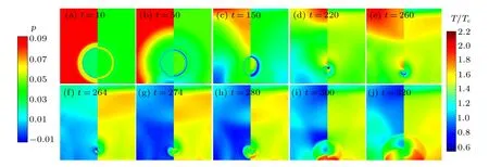
Fig.6. Evolutions of pressure field and temperature field around collapsing bubble near solid wall(case 1).

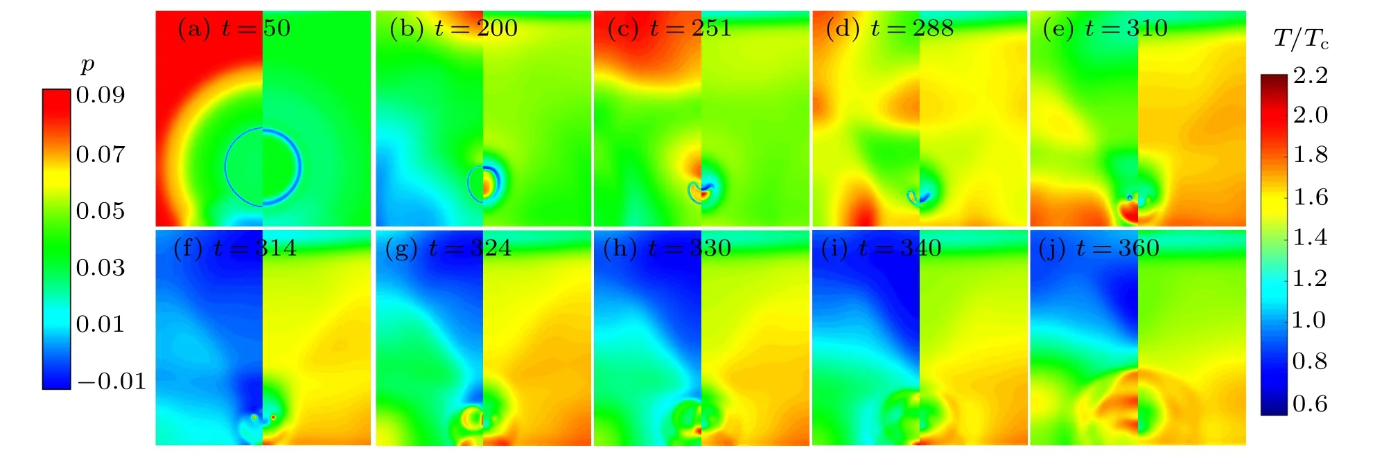
Fig.7. Evolutions of pressure field and temperature field around collapsing bubble near solid wall(case 2).

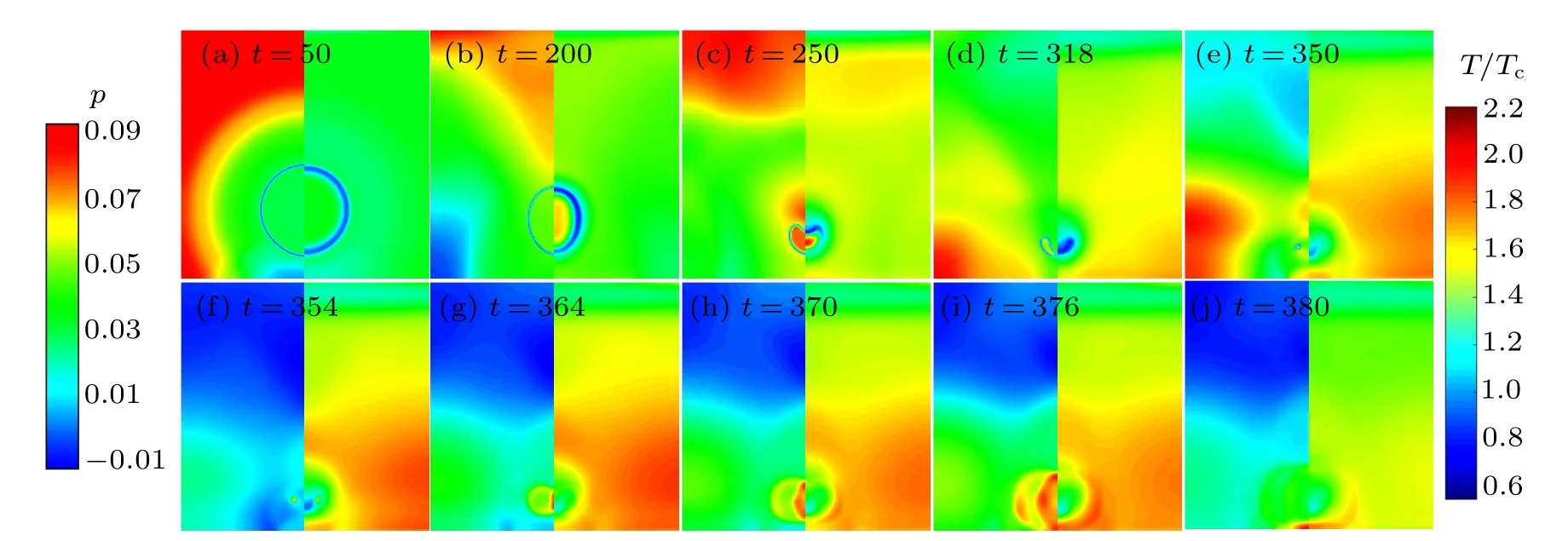
Fig.8. Evolutions of pressure field and temperature field around collapsing bubble near solid wall(case 3).

The above results indicate that the bubbles in all three cases undergo secondary collapse. However, the pressure field, temperature field evolution and collapse velocity of the bubble are different,and the damage to the wall is particularly diverse. Due to the percentage of gas volume in the bubble is the only variable in the simulation, the influencing factor for the cavitation bubble collapse is determined. Furthermore,the damage effects on the wall are analyzed in the following subsection.

4.3. Effects of damage on wall

The crucial roles of pressure and temperature in wall damage are shown by a comparison in Fig.10, which illustrates the time sequences of the two parameters pwand Tw,which are the pressure and the temperature against the rigid boundary,respectively. In order to explain and understand the phenomena shown in Fig.10,the bubble profiles and temperature field images of the first and second collapse are displayed in Fig.9.

As can be seen from Fig.10(a), it is seemed that only one shock wave reaches the solid wall. However,as shown in Fig.9(a), under the same pressure difference, the bubble collapse velocity is fastest in case 1. The volume of the toroidal bubble is relatively small in Figs.9(a1)and 9(b1),so the collapse time of the toroidal bubble is relatively short. The time interval between the two collapses is essentially related to the deformation velocity of the collapsing cavitation bubble,which is also referred to as the collapse time of the toroidal bubble. Therefore,because the time interval between the first collapse and the second collapse is extremely short,the hightemperature and high-pressure shock waves created by the second collapse hit the wall almost simultaneously with the first collapse.

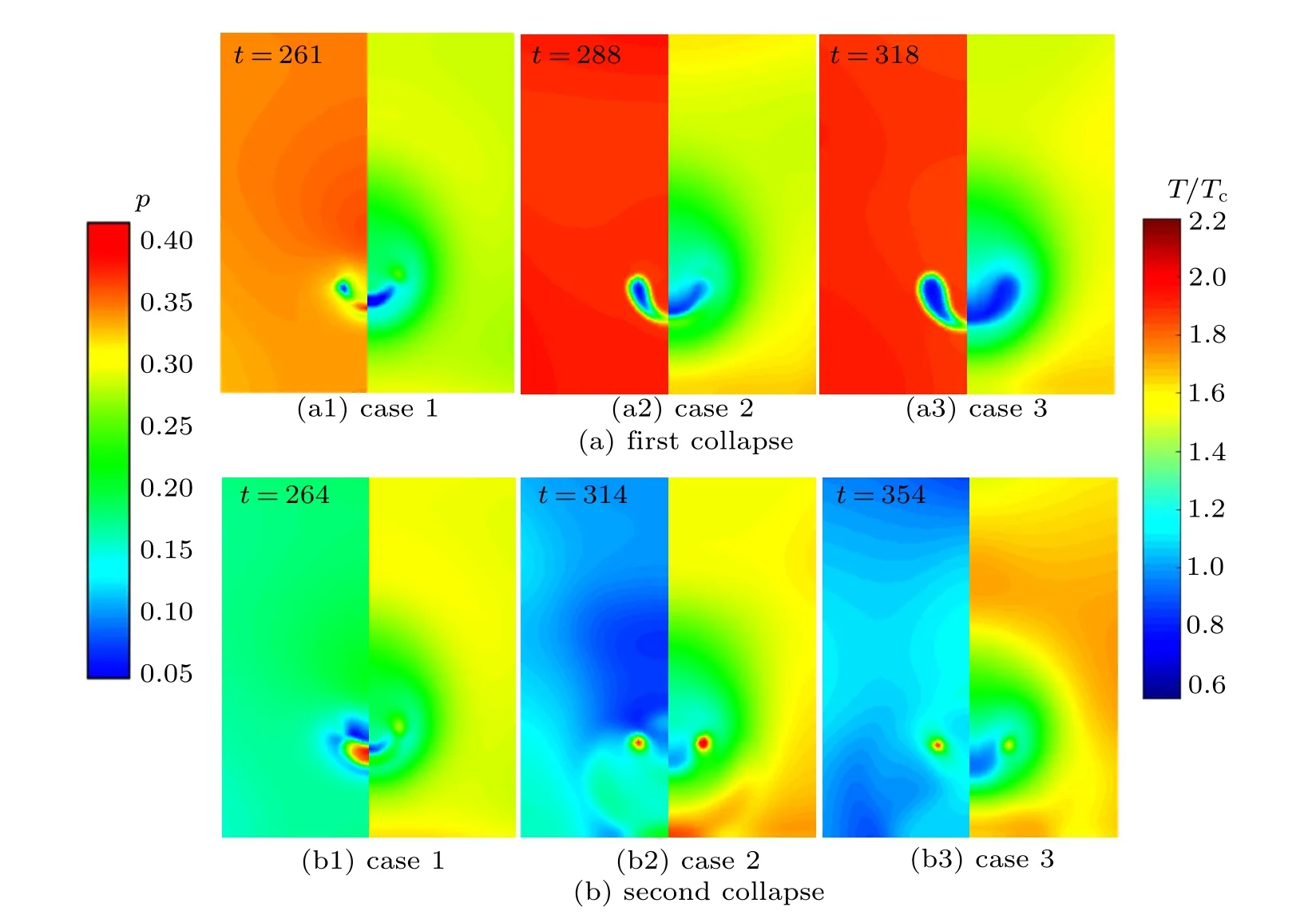
Fig.9. Density field(left)and temperature field(right)at first and second collapse in three cases.

Fig.10. Time sequences of pw and Tw on solid wall for different cases(λ =1.4).

When the volume non-condensable in the bubble is larger,the bubble is not easily broken down by the jet flow, and the time step of the first collapse is longer. This indicates that the non-condensable gas has an impeding effect on the collapsing bubble. A larger volume of the toroidal bubble is shown in Fig.9(a3), and the corresponding collapse time increases.Although the bubble profiles in Figs.9(b2)and 9(b3)are similar, the surrounding density distributions are quite different.As the interval increases, the shockwaves created by the first collapse already rebound off the bottom wall in all directions.There is no timely liquid replenishment in the bottom region near the wall. The pressure waves created by the second collapse hit the wall,driven by the liquid pressure gradient,which causes pwto increase sharply as shown in Fig.10(c). In addition, as the collapse time increases, the temperature dissipation and exchange between the bubble and the surrounding liquid also increase. The internal temperature of the bubble decreases. Therefore,the maximum Twfor case 1 is the highest,and the maximum Twfor case 3 is the lowest in the three cases.

Thus, the non-condensable gas in the bubble can affect the deformation velocity and the profile of the bubble, which results in variations in the thermodynamic and kinetic behavior of the bubble. When the non-condensable gas concentration increases,the distinction of the pressure and temperature on the wall after the second collapse are more obvious. In addition, it is found that the thermodynamic behavior of the bubble is not completely synchronized with the dynamic behavior due to the thermal dissipation in the collapse process that needs further considering.

5. Discussion and conclusions

In this study, a multicomponent thermal MRT-LBM method is adopted to investigate cavitation bubble collapse with non-condensable gas. The temperature changes of the two-component two-phase flow are well-captured by the LBM. Furthermore, it is demonstrated that the multicomponent thermal MRT-LBM method is an effective tool for simulating multicomponent multiphase flow. Some conclusions can be drawn as follows.

(i) The numerical results obtained by the present model comply with the Laplace law and adiabatic law. In addition,the LBM simulation results of cavitation bubble collapse are consistent with the numerical solution of the RP equation for the partial pressure gas.

(ii) A numerical model of cavitation bubble near a solid wall is established. Three cases of different initial volume fractions of non-condensable gas and vapor in the bubble are considered in the simulation to investigate the different morphologies and thermodynamic behavior of collapsing bubble.The pressure and temperature field evolution provide clear physical pictures for understanding the mechanism of bubble collapse near the wall. The results show that the noncondensable gas concentration in the bubble significantly influences the collapse consequence.

(iii) The pressure and temperature against the solid wall during the first collapse and the second collapse are explained by analyzing the bubble profiles of each collapse in detail.When considering the non-condensable gas, the thermodynamic and kinetic behavior of the bubble vary. The distinction of the pressure and temperature on the wall after the second collapse are more obvious as the non-condensable gas concentration increases. Therefore,it is of great importance to study the effect of non-condensable gas inside bubble on cavitation.

The influence of the non-condensable gas in the bubble can provide an insight into the engineering or industry of the cavitation applications. Future work will focus on the cavitation bubble with mixture non-condensable gas and vapor collapse near a thermal/cold wall.