
Control of chaos in Frenkel–Kontorova model using reinforcement learning*
2021-05-24 02:25YouMingLei雷佑铭andYanYanHan韩彦彦
Chinese Physics B 2021年5期
You-Ming Lei(雷佑铭) and Yan-Yan Han(韩彦彦)
1School of Mathematics and Statistics,Northwestern Polytechnical University,Xi’an 710072,China
2Ministry of Industry and Information Technology(MIIT)Key Laboratory of Dynamics and Control of Complex Systems,Northwestern Polytechnical University,Xi’an 710072,China
Keywords: chaos control,Frenkel–Kontorova model,reinforcement learning
1. Introduction
In 1938, the Frenkel–Kontorova (FK) model was firstly proposed by Frenkel and Kontorova to describe the dynamics of a crystal lattice in the vicinity of the dislocation core.[1]Though rather simple,it has the ability to describe many phenomena in solid-state physics and nonlinear physics.[2]It has been used to model dislocation dynamics, surfaces and adsorbed atomic layers, incommensurate phases in dielectrics,crowd ions and lattice defects, magnetic chains, Josephson junctions, DNA dynamics, etc. Generally, the occurrence of chaotic behaviors limits the performance of the model and may cause instability in engineering applications, wear and additional energy dissipation in solid-friction and insufficient output power in electronic applications,so it is of significance to control chaos in the system.[3–7]
Chaos control has been studied for three decades since the pioneering work of Ott, Grebogi, and Yorke.[8]Later on,many control methods were proposed such as the feedback control method,[9–13](non-)linear control method,[14–16]and adaptive control method.[17–19]Most of these methods usually depend on the explicit knowledge of the controlled system. For examples, Yadav et al. used a feedback controller with the assistance of the Routh–Hurwitz condition to suppress three chaotic systems with an exponential term,[13]and Gao et al. designed a linear controller under the known system to control chaos in the fractional Willis aneurysm system with time-delay.[15]Concerning “real world applications”, it is difficult, however, to meet this requirement for the highdimensional dynamical system such as the FK model. On the other hand, Gadaleta and Dangelmayr introduced a reinforcement learning-based algorithm to control chaos where the optimal state-action value function was approximated by Qlearning or Sarsa-learning.[20]The algorithm requires no analytical information about the dynamical system nor knowledge about targeted periodic orbits. They showed that the algorithm was able to control a nine-dimensional Lorenz system by changing its state with proportional pulses. In their further study, they showed that the method was robust against noise and capable of controlling high-dimensional discrete systems,one-dimensional (1D) and two-dimensional (2D) coupled logistic map lattices, by controlling each site.[21]The control policy established from interaction with a local lattice can successfully suppress the chaos in the whole system, and thus forming a new pattern. Their findings might open promising directions for smart matter applications, but future research needs to focus on controlling continuous coupled oscillators as they pointed out. Besides, Wei et al. used an algorithm based on reinforcement learning to realize the optimal tracking control for unknown chaotic systems.[22,23]The advantage of the method is its simplicity and easy implementation.
In the present work, we use the model-free reinforcement learning-based method to control spatiotemporal chaos in the FK model because the method provides a possibility of “intelligent black-box controller”, which can be more directly compatible with the actual system, making the controller very suitable for controlling experiment systems.[21]The control of the FK model has drawn much attention in pursuing friction and wear reduction.[12]Surprisingly, Braiman et al. showed that the introduction of disorder in pendulum lengths can be used as a means to control the spatiotemporal chaos in the FK model.[24]According to the properties of terminal attractors,[11]Braiman et al.proposed a global feedback scheme to control the frictional dynamics of the FK model to the preassigned values whereby only the average sliding velocity is utilized. Brandt et al.showed that appropriate phase disorder in the external driving forces can make the chaotic FK model produce periodic patterns.[25]In view of these facts,we exert an optimal perturbation policy on two different kinds of parameters, i.e., the pendulum lengths and phases, based on the reward feedback from the environment that maximizes its performance. In the training step, the optimal state-action value function is approximated by Q-learning and recorded in a Q-table. Note that in the Q-table we only consider the mean velocity of all oscillators in the FK model since it is usually a macroscopic quantity and easily observed. In the control step,the optimal control action according to the Q-table is selected and then applied to controlling pendulum lengths or phases of the system,respectively.
The rest of the paper is organized as follows.In Section 2,we briefly introduce the FK model, presenting a model-free control algorithm, and employing the algorithm to suppress chaos in the FK model based on the reinforcement learning.In Section 3, the proposed method is used to implement the numerical simulations for two different kinds of policies,i.e.,changing pendulum lengths and changing phases,respectively.In particular,we modify the control strategy with pining control, that is, only control a small number of oscillators in the FK model. Finally,in Section 4 we present some conclusions and discussion.
2. Chaos control of FK model through RL
2.1. FK model

In this work,we attempt to control spatiotemporal chaos in the FK model. The standard FK model can be seen as 1D lattice of identical pendulums oscillating in the parallel planes, coupled to the nearest neighbors by the same torsion springs. Braiman et al.generalized the model to a coupled array of forced,damped,nonlinear pendulums.[24]The equation of motion we consider can be described by where θnis the angle of the pendulum and= dθn/dt,= d ˙θn/dt, lnis the pendulum length, ϕnis the phase angle (n=1,2,...,N). And free boundary conditions are considered,i.e.,θ0=θ1,θN+1=θN. Parameters are set to be the pendulum bob m=1.0,the acceleration due to gravity g=1.0,coupling κ =0.5,direct current(DC)torque τ′=0.7155,alternating current(AC)torque τ=0.4,the damping coefficient γ =0.75, and the angular frequency ω =0.25. The dynamic behavior of the FK model is chaotic for the default phase angle ϕn=0 and the default length ln=1.0,which is characterized by a positive Lyapunov exponent.[24]
2.2. Model-free RL algorithm
In the model-free RL algorithm, the agent’s perception and cognition for the environment is realized only through continuous interaction with the environment. The data obtained by the agent interacting with the environment are not used to model the environment, but optimize the agent’s own behavior. This solves the problem that the explicit knowledge of the FK model is difficult to obtain when the FK model is taken as the interactive environment in RL algorithm.
The aim of RL is to find an optimal policy that maximizes the accumulated reward successfully accomplishing a task by interacting with the environment. In each step of the episode,the agent receives the environment’s state snand the agent selects an action unbased on sn.The action is selected according to a policy π,which is described by a probability distribution πn(s,u)of choosing un=u if sn=s.Then the environment executes the action unand outputs an immediate reward rn+1and a new state sn+1to the agent.By doing so,the learning method offered by RL algorithms improves the policy that associates with the environment’s state through observations of delayed rewards so that the rewards are maximized over time. Repeating such process for different episodes and travelling through the state space,we can obtain at the end the expected optimal policy which allows for controlling spatiotemporal chaos.
In this work,Q-learning,a learning method of the modelfree RL algorithms which was proposed by Watkins,[26]is used to improve the policy in each time step,so that the accumulated rewards with the discounted γ ∈[0,1]are maximized as follows:

Usually, the problem with delayed reward can be modelled as a finite Markov decision process (MDP). The MDP includes a set of states s ∈S and actions u ∈U,a state transition function Pu(sn+1, sn)specifying the probability of a transition from state snto sn+1using action u,and a reward function R(s,u)denoting the expected immediate reward function of the current state s and action u. Additionally, the learning method for the MDP computes optimal policies by learning a state-action value function. The state-action value function Q:S×U →R gives the Q value of a state-action pair (s,u)under a certain policy π as
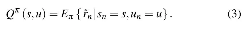
For any state s and any policy π, equation(3)can recursively be defined on the basis of the Bellman equation
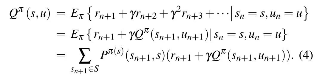
To receive the rewards,the Q function in Eq.(4)for all(s,u)is maximized under an optimal policy π*such that the best solution Q*=Qπ*satisfies the Bellman optimality equation in the following form:[27]
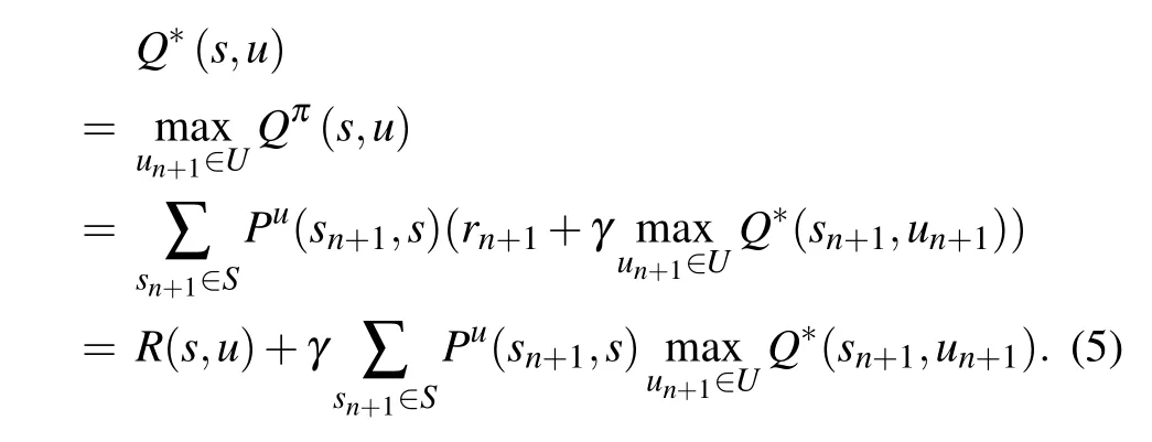
We denote by H(Q) the operator on the right-hand side of Eq.(5). For unknown R(s,u)and Pu(sn+1,sn),H cannot be determined,so the solution of Qn+1=H(Qn)can be approximated by the stochastic Robbins Monroe algorithm[27–29]

2.3. Control of chaos in FK model by using model-free algorithm
In this subsection, we consider controlling spatiotemporal chaos in the FK model using the model-free RL algorithm.In the algorithm,we require no explicit knowledge of the FK model, but need a simulation environment to interact. Therefore,we must identify the key elements in RL including states,actions,and reward function before the algorithm is employed.

After determining the states that the agent can obtain,the deterministic policy π*is used to choose an action u under a current state s in each time step in that the action corresponding to the maximum Q value is appropriately chosen. When Q values under the current state are equal, the action is randomly chosen,which ensures the exploration of the whole action space.The selected action is then input into the FK model and acts on controllable parameters in the system. These controlled parameters are selected only if they have certain practical significance. In Eq.(1),the controlled parameters are the phase angle ϕnand the length lnthat can be manipulated.With regard to the parameters,we can obtain a corresponding action space{u1,u2,...,uM}.
The Q values of a state-action pair (s,u) are stored in a single table, Q-table that is directly updated through Eq. (8)leading to the optimal policy for all the states. The Q-table is a matrix requiring the state space S and the action space U to be finite and discrete. In order to make the state space S satisfy these requirements,we divide the interval of all possible states of the system into finite points,where their midpoints,as reference states, constitute the state space S. The state space S is comprised of 1D discrete points,and its elements are given in advance through the uncontrolled system. Specifically, we can determine the interval of the possible mean velocity’s local minimums after entering chaos through the uncontrolled system, and then uniformly discretize it into different reference states that form the state space S ⊆R. By doing so,each state obtained from the system needs to be mapped to a reference state in the state space in the process of learning.


Fig.1.Illustration of controlled FK model by Q-learning where sn and un represent current state and control input of the model,and sn+1 and rn+1 denote next state and immediate reward.

Fig.2. Flowchart of controlling chaos in FK model by using RL algorithm.
When Q-learning is used to control chaos in the FK model,the relationship among these key elements is illustrated in Fig.1. The goal of the task is to maximize the value function Q. We explore the environmental FK model and update the Q-table based on the reward function. With the aid of the Q-table, we seek the best action at each state by exploiting the FK model. The Q-table keeps updating through Eq.(8)as shown in the right part of the figure,and returns the expected future reward.
A flowchart of the whole learning algorithm is shown in Fig.2.In the learning process,we infer and record the controllable parameters of the FK model at each state,so we can use the real-time control method to realize the purpose of transferring chaos to periodic orbits. This method is an online control strategy in RL algorithm,which requires setting a random initial state before the controller works and then updating the Q-table. Naturally, the Q-table is initialized to a zero matrix because the agent knows nothing about the system before control. In this study,N is the number of states,M is the number of actions, I is the maximum step of an episode, and J is the maximum number of episodes. In particular,we suppose that the control fails and the program exits when j >J.This avoids the problem of an infinite loop in the program when the task cannot be accomplished even though we can always control chaos in the FK model for 100 random initial states.
3. Numerical simulations
The model-free RL algorithm introduced in the previous section is tested on the 1D coupled nonlinear pendulums—the FK model. It is explicit to exhibit spatiotemporal chaos, thus providing a suitable experimental platform for the proposed control approach. In this section, we show the dynamics of the FK model in the phase space,and employ the perturbation policy on two different kinds of parameters,i.e.,the pendulum lengths and the phase angles,to control chaos of the model using RL algorithm.
3.1. Spatiotemporal chaos in uncontrolled system
We consider the 1D coupled array of forced, damped,nonlinear pendulums shown in Eq. (1). We numerically integrate the equations of motion by using the fourth-order Runge–Kutta algorithm in steps of dt =T/2500, where T =2π/ω, ω =0.25, and initial values of the angles and angular velocities are randomly chosen in the intervals [−π, π]and [−1, 1], respectively. The time history of the uncontrolled system,the continuous spatiotemporal system of an array of N=128 pendulums,and its mean velocity are plotted in Fig.3,where the colors represent the values of angular velocity ˙θn. When the default length ln=1.0 and the default phase ϕn=0.0 for all the driving forces,we calculate the largest Lyapunov exponent of the average velocity through a data-based method,which identifies the linear region by the density peak based clustering algorithm.[30,31]When the sampling step is 0.1 and the length of the time series is 105, the largest Lyapunov exponent is 0.3134. This means that the uncontrolled FK model stays in a chaotic attractor.
From Fig. 3(a), it can be observed that the local minimums of the mean velocity of the angular velocities of oscillator appear aperiodic and stay in the interval[0.1, 0.3]after 60T transient states.In fact,the result shown in Fig.3(a)is just one of 100 initial values that we randomly select. The minimum values of the average velocity under other initial values also fall into an approximate interval. Figure 3 shows that the FK model appears to be spatiotemporally chaotic. To characterize the Q-table’s rows,we choose 200 reference states uniformly distributed between 0.1 and 0.3 as the elements of the state space. The agent maps each state min(¯v(t))obtained from interaction with the FK model into the state space in which the projection is defined as

Besides, the available parameters, the pendulum lengths or the phase angles,are used to establish the control policy in controlling the coupled pendulums with spatiotemporal chaos.For the two different parameters, we take into consideration the global control strategy, which changes all of the lengths or phase angles, and the pinning control strategy, which only alters a small number of lengths or phase angles,respectively.

Fig. 3. Spatiotemporal evolution of an array of N =128 coupled pendulums: (a) evolution of mean velocity ¯v(t) and (b) spatiotemporal evolution of angular velocities,with parameters set to be g=1.0,m=1.0,γ =0.75,τ′=0.7115,τ =0.4,κ =0.5,ln=1.0,and ϕn=0.
3.2. Changing lengths
In this subsection, we adopt the model-free RL algorithm in Section 2 to control chaos in the FK model by changing the pendulum lengths with the global and local pinning control strategy, respectively. Previously, Braiman et al. introduced 10% or 20% randomly disorder into all of the pendulum lengths, successfully taming the spatiotemporal chaos.[24]In view of this, we select the action u ∈U ={−0.2, −0.1, 0.0, 0.1, 0.2} exerted on the lengths ln, n =1,2,...,128, and thus the Q-table becomes a 200×5 matrix,in which the rows represent the 200 reference states s ∈S and the columns refer to the available 5 control actions u ∈U. As a criterion for control, we apply the action to the pendulum lengths whenever the mean velocity of the model reaches a local minimum, i.e., ln→ln+u if ¯v is at a local minimum. To ensure the system entering into chaotic behaviors, we implement the control strategy after discarding 60T transient states.
In the learning algorithm, we set the maximum number of steps to be I = 500, when the number of steps i >I in an episode,executing the next episode,and set the maximum episode to be J=300,when the number of episodes j >J,the control fails and the program exits.

Fig.4. Time history of an array of N=128 coupled pendulums with global control strategy by changing pendulum lengths: (a) evolution of mean velocity (t),and(b)spatiotemporal evolution of angular velocity.
With the global control strategy for the pendulum lengths,we apply the same control action u to all of the pendulum lengths once the mean velocity reaches a local minimum. The time history of the mean angular velocity and the spatiotemporal evolution of an array of 128 pendulums with the global control strategy on the pendulum lengths are shown in Fig.4 where the initial values of the angles and the angular velocities are randomly chosen in the intervals[−π, π]and[−1, 1],respectively. Comparing with the case without control in Fig.3,figure 4(a)shows that the mean velocity of the controlled FK model changes periodically and figure 4(b) shows that the model with an initial value presents a non-trivial,periodic pattern after a disordered transient states if the control is turned on. To check whether the chaotic system is successfully suppressed, we calculate the largest Lyapunov exponent of the controlled FK model and it is −0.1316,which verifies further that the controlled system is not chaotic and stays in a regular pattern. This means that the model-free RL method can suppress spatiotemporal chaos in the FK model by changing all the pendulum lengths when part of the average velocity can be observed.

Fig.5. Error of e angular velocity versus time,indicating all of the pendulums are synchronized with time evolution by changing pendulum lengths.
Interestingly,we show in Fig.4(b)that all the pendulums are synchronous in space. So,we define an error between the mean velocity and those of all the pendulums
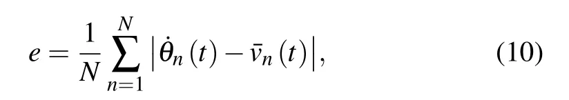
to quantify this phenomenon. As can be seen in Fig. 5, the error in the model with control tends to zero very quickly. It is shown that the 128 pendulums’angular velocities are completely consistent with the average velocity,that is,these pendulums under the current control strategy will be synchronized very quickly. The synchronous phenomenon was not found in Ref. [24] because the method of introducing disordered pendulum lengths into taming spatiotemporal chaos might exert different influences on different pendulums. Notice that in Ref. [24] the system appears to be spatiotemporally chaotic if all of the pendulum lengths are fixed to be ln=1.0 while it may generate a regular pattern if all of the pendulum lengths are different. It should be pointed out that although all of the pendulums in that case have the same lengths,the pendulums with different initial values are chaotic, but not synchronous;while in this case, all of the pendulums with control will finally fall into the same periodic orbit and be synchronous in that the reward function we design continuously guides each pendulum to following the same mean trajectory of the system by simultaneously changing the pendulum lengths using RL algorithm.
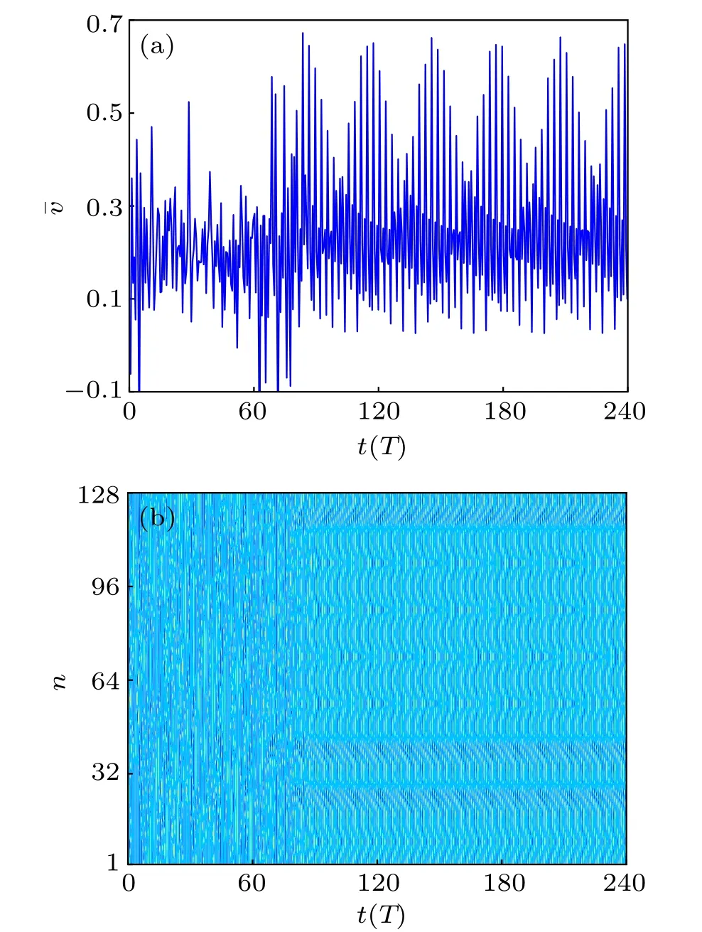
Fig. 6. Time history of an array of N =128 coupled pendulums with pinning control strategy by changing 8 pendulum lengths:(a)evolution of mean velocity ¯v(t)and(b)spatiotemporal evolution of angular velocity.
In the global control strategy,all of the pendulum lengths in the FK model need to be under the same real-time control, which is usually difficult to employ in practical applications. So, we modify this strategy and introduce a pinning control one, which only selects a small number of pendulums to change their lengths, to suppress chaos in the model.Therefore,we divide 128 pendulums into eight equal parts and choose one pendulum in each part with equal spatial intervals.By doing so, we exert the control action u on 8 pendulums and change the lengths of the corresponding pendulums by the model-free RL method. The behavior of the mean angular velocity and the spatiotemporal evolution of an array of 128 pendulums with the pinning control strategy on the pendulum lengths are shown in Fig.6 where the initial values of the angles and the angular velocities are randomly chosen in the intervals [−π, π] and [−1, 1]. Like Fig. 4, the mean velocity under the control manifests a periodic behavior after a transient state in Fig. 6(a) and the controlled FK model immediately presents a regular pattern in Fig.6(b)while turning on the control. At this time, the largest Lyapunov exponent of the model is −0.1186, so the pinning control strategy by changing pendulum lengths can suppress chaos in the model.Unlike the previous case,the pendulums of the system in this case are temporally periodic, but not spatially synchronized.In this sense,the controlled system presents much richer patterns,making various types of regular patterns generated more easily. By comparison, the patterns induced by the pinning control strategy show a kind of lag synchronization.
Besides, in order to verify the effectiveness of the proposed method, we select 100 different initial values for the policies.It is found that for all of the initial values the chaos in the FK model can be suppressed. Therefore,we conclude that both the global control strategy and the pining one using the model-free RL method by changing the pendulum lengths can make the chaos in the FK model suppressed and give rise to regular patterns. By comparison,the latter one usually makes the controlled system generate much richer patterns,of which the form depends on the initial angular displacements and velocities.
3.3. Changing phase angles
In this subsection,we employ the RL control technique to suppress chaos in the FK model by changing the phase angles with the global and pining control strategy, respectively. The action space is U = {−π, −0.5π, 0.0, 0.5π, π}, in which the action u ∈U is exerted on the phase angle ϕn. As a criterion for control,we apply the action to the phase angles whenever the mean velocity of the model reaches a local minimum after discarding transient states. That is,we let ϕn→ϕn+u if the mean velocity ¯v arrives at a local minimum where u ∈U is chosen according to the RL algorithm-based control strategy.
With the global control strategy by changing the phase angles ϕn,the action u is acted on all of the phase angles in each step of an episode. The behavior of the mean velocity and the spatiotemporal evolution of an array of 128 pendulums with the global control strategy for the phase angles are presented in Fig.7 where the initial values for the angles and the angular velocities are randomly chosen in the intervals[−π, π]and[−1, 1]. It is shown that the mean angular velocity of the controlled system changes into being periodic in Fig.7(a),and the 128 pendulums quickly fall into periodic orbits in time and are synchronized in space in Fig.7(b)if the control is turned on.In addition, the largest Lyapunov exponent of the controlled system is−0.1933. This verifies further that the spatiotemporal chaos in the array of 128 pendulums can also be suppressed by varying all the phase angles,which is easier in practice than by changing the pendulum lengths.
In the same way, the pinning control strategy is implemented by changing a small part of the phase angles ϕn. In analogy with the process in the previous subsection,we divide 128 pendulums into eight equal parts and choose one pendulum in each part with equal spatial intervals to change its phase angle using the model-free RL algorithm. The behavior of the average velocity and the spatiotemporal evolution of the array of 128 pendulums are illustrated in Fig. 8. As we can see,the mean velocity under the control manifests a periodic behavior after a transient state and the controlled FK model immediately presents a temporally periodic pattern with spatial lag synchronization of pendulums. Besides, the largest Lyapunov exponent of the controlled FK model is −0.1035. So,we can obtain that the pinning control strategy by changing only a small part of phase angles can be put into effect and suppress chaos in the FK model,which provides a more feasible way since altering phase angles is easier to implement than altering pendulum lengths.
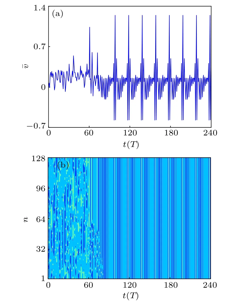
Fig.7. Spatiotemporal evolution of an array of N=128 coupled pendulums with global control strategy by changing excitation phase: (a) evolution of mean velocity ¯v(t)and(b)spatiotemporal evolution of angular velocity.
As stated above, 100 initial values are randomly chosen.We show that none of the initial values affects the main conclusion and chaos of the FK model can always be suppressed regardless of selected initial values, indicating that altering phase angles using the model-free RL algorithm can indeed tame spatiotemporal chaos. More importantly, changing the phase angles with the global control strategy can make all of the pendulums in the FK model synchronized completely,which could not be shown in Ref.[25]. This is because all of the pendulums with the global control are slaved to follow under the guide of the reward function the trajectory of the mean velocity of the FK model, and thus finally reaching the same periodic orbit,while in the latter case introducing phase disorder by modifying the driving forces only makes the majority of regular pendulums dominate over the remaining chaotic ones so that the whole system transfers from chaotic to kind of synchronous,regular pattern.
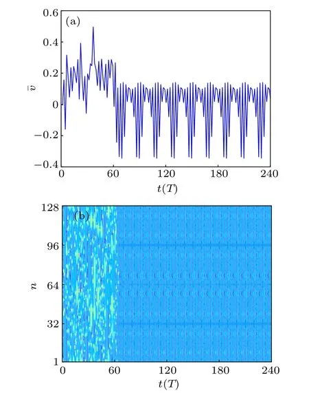
Fig.8. Spatiotemporal evolution of an array of N=128 coupled pendulums with pinning control strategy by changing 8 excitation phases: (a) evolution of the mean velocity ¯v(t) and (b) spatiotemporal evolution of angular velocity.
4. Conclusions and discussion
In this work,we generalize the model-free reinforcement learning method to control spatiotemporal chaos in the FK model. The advantage of the method is that it does not require analytical information about the dynamical system and any knowledge of targeted periodic orbits. In the method,we use Q-learning to find optimal control strategies based on the reward feedback, and determine the local minimums of the mean velocity of the pendulums in the FK model from the environment that maximizes its performance. The optimal control strategies are recorded in a Q-table and then employed to implement controllers. Therefore, all we need is the parameters that we are trying to control and an unknown simulation model that represents the interactive environment given observed mean velocity of all of the pendulums in the FK model.Here we apply the perturbation policy to two different kinds of parameters, i.e., the pendulum lengths and the phase angles of excitations. We show that both of the two perturbation techniques,i.e.,changing the lengths and changing their phase angles, can suppress spatiotemporal chaos in the system and make periodic patterns generated. In particular,we also show that the pinning control strategy, which only changes a small number of lengths or phase angles,can be put into effect. The proposed method is an intelligent black-box method and meets simple requirements in practical applications such as the nonlinear physics,the solid-state physics,and the biology,so that it can provide a possible control strategy for high-dimensional chaotic systems in the real world.

- Chinese Physics B的其它文章
- Corrosion behavior of high-level waste container materials Ti and Ti–Pd alloy under long-term gamma irradiation in Beishan groundwater*
- Degradation of β-Ga2O3 Schottky barrier diode under swift heavy ion irradiation*
- Influence of temperature and alloying elements on the threshold displacement energies in concentrated Ni–Fe–Cr alloys*
- Cathodic shift of onset potential on TiO2 nanorod arrays with significantly enhanced visible light photoactivity via nitrogen/cobalt co-implantation*
- Review on ionization and quenching mechanisms of Trichel pulse*
- Thermally induced band hybridization in bilayer-bilayer MoS2/WS2 heterostructure∗