
A modified analytical model of the alkali-metal atomic magnetometer employing longitudinal carrier field*
2021-05-24 02:22ChangChen陈畅YiZhang张燚ZhiGuoWang汪之国QiYuanJiang江奇渊HuiLuo罗晖andKaiYongYang杨开勇
Chinese Physics B 2021年5期
Chang Chen(陈畅), Yi Zhang(张燚), Zhi-Guo Wang(汪之国),†, Qi-Yuan Jiang(江奇渊),Hui Luo(罗晖), and Kai-Yong Yang(杨开勇)
1College of Advanced Interdisciplinary Studies,National University of Defense Technology,Changsha 410073,China
2Interdisciplinary Center for Quantum Information,National University of Defense Technology,Changsha 410073,China
Keywords: alkali-metal atomic magnetometer,longitudinal carrier magnetic field,linear-response capacity
1. Introduction
Alkali-metal atomic (AMA) magnetometers[1,2]using parametric modulation can achieve ultrahigh sensitivity in the order of nT–fT, due to the advantages of the synchronous demodulation techniques and suppression of low-frequency flicker noise. They have been demonstrated for the detection of biomagnetic signals from the human body,[3]magnetic resonance imaging (MRI),[4]fundamental physics study,[5]the detection of low-field nuclear magnetic resonance (NMR)[6]and other applications. The AMA magnetometer employing an oscillating carrier magnetic field along the z-axis as the longitudinal direction, was first devised in Ref. [7] and used to detect3He nuclear polarization.[8]Later, by applying a static magnetic field and optical pumping light along the same direction of the carrier field, this magnetometer technique was developed and used in spin-exchange[9,10]NMR oscillators or gyroscopes,[11,12]as a vector magnetometer that is maximally sensitive to the low-frequency and very weak magnetic fields BTin the x–y plane caused by the processing nuclear magnetization vector in the alkali vapor cell, and insensitive to Bzalong the rotation axis of the gyroscopes.[13]
Following the derivations in Ref.[7],the analytical models presented in Ref.[12]describe the rubidium magnetometer signal that is only proportional to small magnetic fields Bxand Bywithin the linewidth of the rubidium magnetization vector, because it is assumed that the longitudinal component of the rubidium magnetization Mzis constant. Reference [14]demonstrated a two-transverse axis atomic magnetometer by utilizing parametric modulation of the z-magnetic field and operating in the spin-exchange relaxation-free regime, under the condition that they also approximated the z-component of the Rb atomic spin polarization Szis S0, which is determined by optical pumping and any magnetic-field-induced changes can be neglected. References [12,14] mainly considered the sensitivity of the magnetometer and they have done little research on its linear-response characteristics. Reference [15]demonstrated a three-axis atomic magnetometer employing longitudinal field modulation,which can not only measure the transverse components, but the longitudinal z-component of the external magnetic field,by extraction from the modulation frequency that tracks the resonance frequency. They modified the expression of the quasi-static magnetic field Btotto explain the reducing orthogonality of the magnetometer for larger transverse fields. However, there are considerable differences between their modified theoretical curve and experimental curve of the magnetometer response when Bxand Byare larger than 100 nT. In practice, we cannot ignore that the longitudinal magnetization Mzwill be influenced by and vary with the magnetic fields BTin the x–y plane, especially for a large measuring range.
In this work, we study the problem of how large magnetic fields in the x–y plane influence the longitudinal magnetization Mzand study the linear-measurement characteristics of the magnetometer within a relatively large range of BT.We give a detailed and rigorous theoretical derivation by using the perturbation-iteration method to obtain a modified analytical model of this magnetometer. The simulation experiment results are presented to verify our theoretical model.This work will help us to find the factors that influence the linearresponse capacity of the magnetometer and configure proper working conditions for a practical measuring system.
2. System setup
A schematic of a typical apparatus of this type of AMA magnetometer is shown in Fig. 1. The sample cell made of glass is placed in magnetic shields, containing a few milligrams of alkali metal and some buffer gas or noble gas. The cell is heated by hot air or non-magnetic electronic heaters driven by high-frequency AC currents, to ensure sufficient number density of alkali-metal atoms.The sum of all of the individual alkali spins in the vapor cell can be represented by the macroscopic magnetization vector M =(Mx,My,Mz) in the xyz-laboratory coordinate system.Uniform static field and carrier field are applied along the z-axis, Bz=B0+Bccos(ωct).A beam of strong circularly polarized laser tuned to an atomic resonance is applied to transmit through the vapor cell along the z-axis,to polarize the alkali spins by optical pumping.[16]A beam of weak linearly polarized laser tuned near an atomic resonance is applied to transmit through the vapor cell along the x-axis and detected by a photodetector, to sense the xcomponent of the alkali spin polarization Mxby the Faraday optical rotation method.[17]The output of the detector is sent to a signal processing system to extract the Bxand Byinformation from the modulated signal Mx.
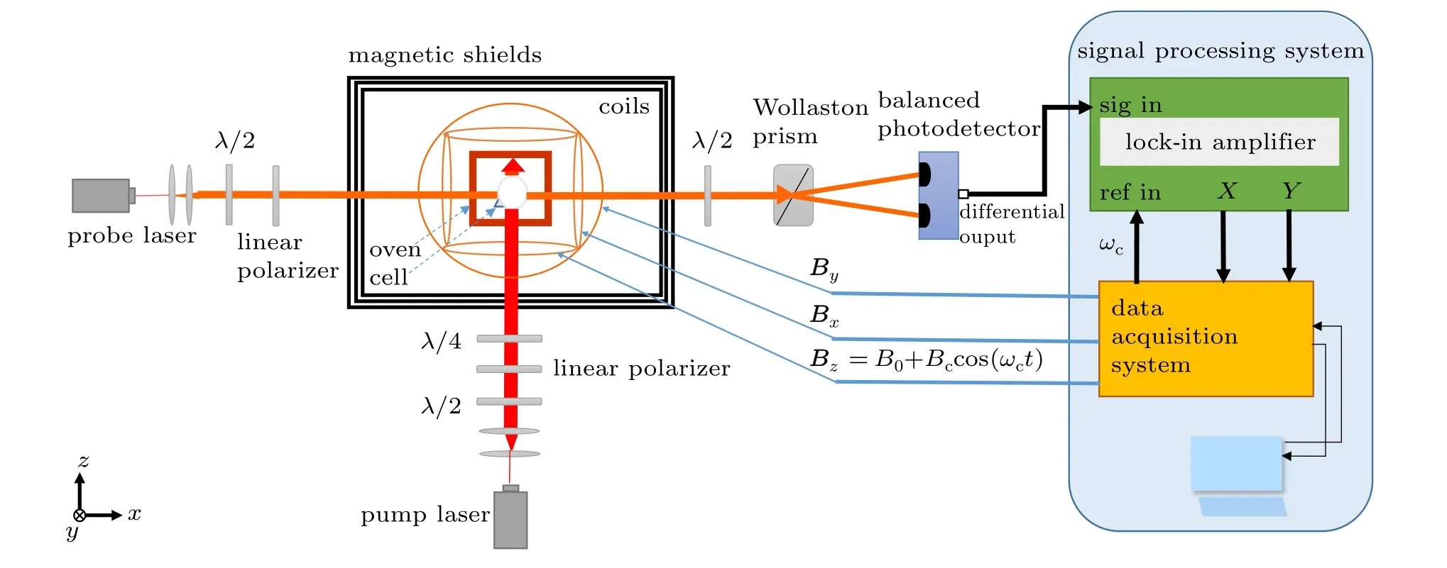
Fig.1. Schematic of a typical apparatus of an alkali-metal atomic magnetometer employing a longitudinal carrier magnetic field.
3. Theoretical derivation
When the magnetization vector M interacts with the external magnetic fields B=(Bx,By,Bz)and the optical pumping light,the dynamics of the magnetization can be described by the Bloch-like equation[7]

where,x,y and z are the unit vectors along the x,y and z axis,respectively;γ is the gyro-magnetic ratio of the alkali spin;M0is the longitudinal z-component of the magnetization of alkali spins in the equilibrium state when optical pumping is on, τ1and τ2are the longitudinal relaxation time and the transverse relaxation time of alkali spins, respectively, which are the total time constants that include both the optical pumping and relaxation effects.[18]Under normal conditions,optical pumping is much stronger than the relaxation, and τ1and τ2are in the order ofµs–ms.
Assuming that the slowly varying magnetic fields to be measured are along the x-axis, By= 0. By setting M+=Mx+iMy,equation(1)now can be written as

where ω0=γB0and ω1=γBc.
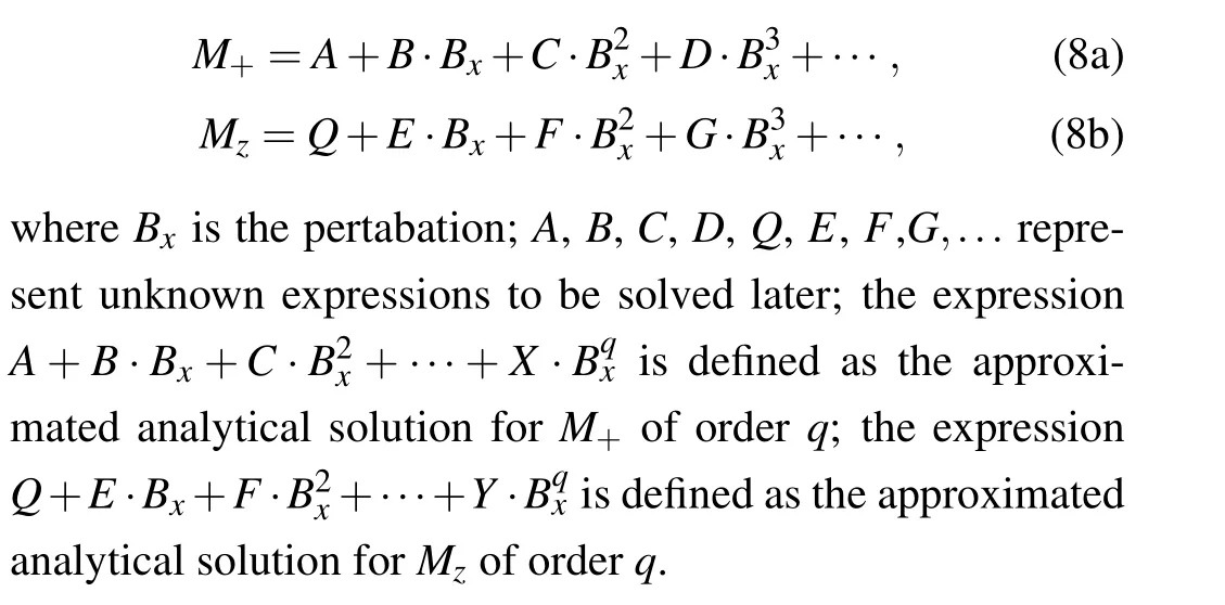
When ωc≫1/τ2(the frequency of the modulation field is much higher than the spin relaxation rate), magnetization M+cannot respond to the modulation field synchronously and will oscillate at various harmonics of modulation frequency ωc(i.e.,M+contains high-frequency components).
3.1. The fundamental analytical model
First of all, we give a brief introduction of the existing fundamental model describing the working principle of this type of AMA magnetometer.
It can be seen that Mxis composed of the various harmonics of modulation, where each signal of pωcresonates at ω0+nωc=0 and the width is Δω0=2/τ2.
The fundamental model describing the magnetometer signal given by Eq.(7a)shows that,under the condition that the amplitude of the measured magnetic field Bxis very small,the longitudinal magnetization Mz≈M0.Therefore,the amplitude of the magnetometer signal δMxis proportional to the magnetic fields Bx.Hence,Bxcan be extracted from the δMxsignal by in-phase or quadrature demodulation at harmonic pωc.
3.2. The modified analytical model
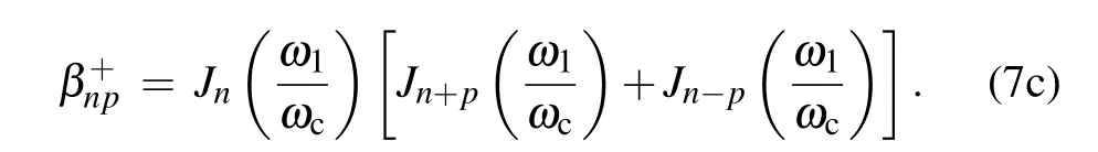
Now,we apply the perturbation-iteration method to solve Eqs.(2a)and(2b).Assuming that M+and Mzcan be expanded as a power series of Bx,let
In Eq.(2b),let Bx=0,and we have

We consider the steady-state solution, setting Eq. (9)equal to zero,and we obtain
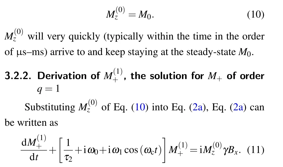
For the same reason as in Subsection 3.1, the quantityin Eq.(11)can be treated as a constant quantity compared to the modulation fields. Under these conditions,by the same method as in Subsection 3.1,we can obtain the analytical


where δMyis the modulation part.
By the same method as in Subsection 3.2.3, substituting the DC term of Myin Eq.(26)and Mzin Eq.(25)into Eq.(2b),we find that the resulting equation satisfies the conditions for a steady-state solution exactly,
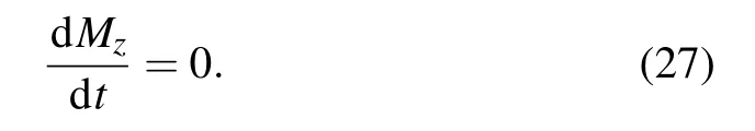
Therefore, we are assured that Eq. (25) can be used as an approximate steady-state solution for Mzunder the condition τ1τ2γ2·J ≥1. Finally,we obtain the general analytical model describing the relationship between Mzand Bx.It can be seen that when the amplitude of the measured magnetic fields Bxis large enough,the value of Mzwill be significantly influenced by Bx;as the amplitude of Bxincreases,the value of Mzdecreases.
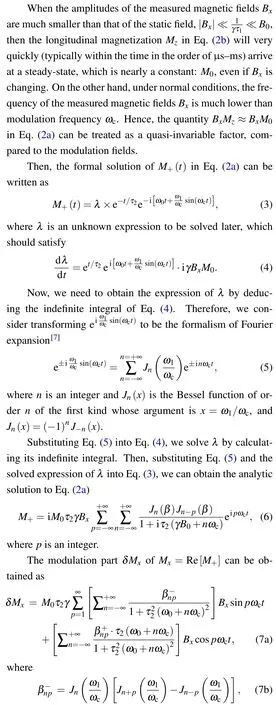
Substituting the solution for Mzof Eq.(25)into Eq.(2a),we can solve the equation and obtain the magnetometer signal Mxand the modulation part δMxwhich is given by
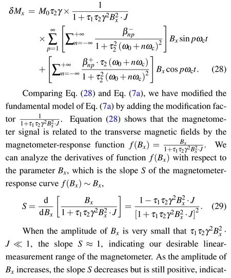

According to Eq.(28),the linear-measurement characteristics of the magnetometer have relationships with these working conditions:the amplitude and frequency of the carrier field determining the value of J, longitudinal spin relaxation time τ1and transverse spin relaxation time τ2;the carrier fields can also influence the spin relaxation time.[19]In order to minimize the influence of a large Bxon the value of the modification factor,the smaller the values of J and τ1τ2,the higher the linear-response capacity of the magnetometer.
4. Numerical simulation and discussion
To demonstrate the validity of our theoretical modification of Eq.(28),we carry out numerical simulation according to Bloch Eq.(1)with our own simulation system constructed by LabVIEW software. The block diagram of the simulation system is shown in Fig. 2. The values of the parameters can be set by inputting to Bloch Equation Solver in the simulation system, incorporating the magnetic fields applied along three axes,the longitudinal and transverse spin relaxation time. The Bloch Equation Solver outputs the values of Mx, Myand Mzof alkali spins. After being amplified in the gain module, the Mxsignal is multiplied by the reference signal of longitudinal carrier fields with a certain phase delay and then processed in the low-pass filter to generate the in-phase or quadrature demodulation results.

Fig.2. Block diagram of the simulation system.
The main parameters are as follows: B0=10 µT, γ =2π×3499 Hz/µT (the alkali metal is133Cs). We consider quadrature demodulating the first (p = 1) harmonic of the magnetometer signal Mxand other parameters for different design examples are given in the specific simulations:
4.1. The n=–1 modulation for different amplitudes of the carrier magnetic field
We set ωc=ω0=γB0; τ1=200 µs, τ2=100 µs. In Eq.(28),as ωc≫1/τ2,and the resonance condition ω0−ωc=0 is satisfied for certain parametric modulation, we can only consider the resonances at n near −1. The condition that ωc≫1/τ1is also satisfied. The parameter of Bcwill be assigned different values. We measure the magnetometer signal response and longitudinal magnetization as the amplitude of the static field Bxis scanned.
The simulation results and corresponding approximate results of the modified analytic solution are shown in Fig.3.It is clear that the theoretical results agree well with the simulation results.
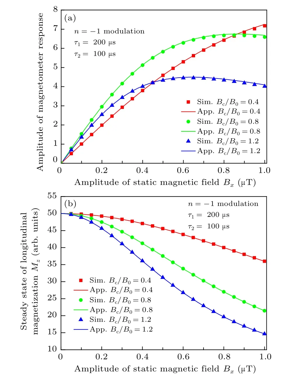
Fig. 3. Magnetometer output for n=−1 modulation under different conditions of amplitudes of the carrier magnetic field:(a)the amplitude of magnetometer response;(b)the steady state of longitudinal magnetization Mz. “Sim.” and“App.” in the figure denote numerical simulation and approximate analytical results,respectively.
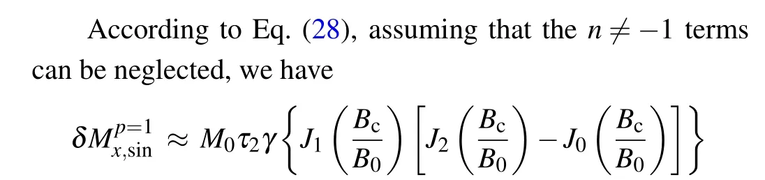
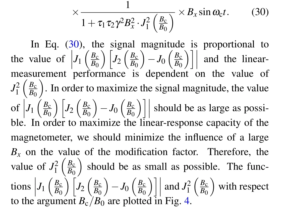
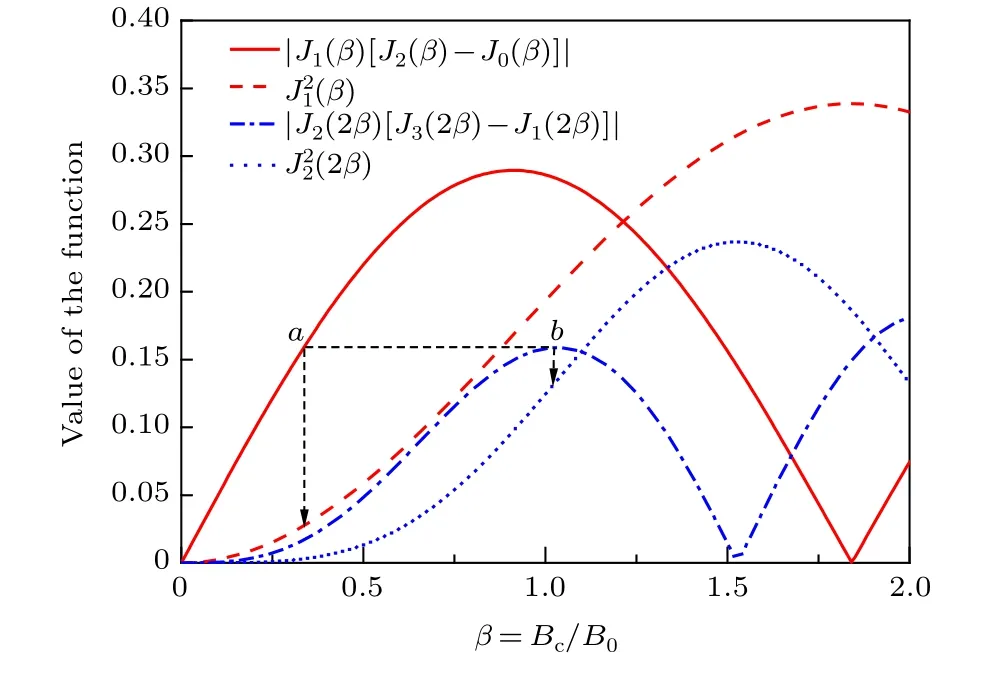
Fig. 4. Functions combined according to Eqs. (30) and (32) plotted against β =Bc/B0.

It can be seen that the relative error depends on the relaxation time τ1τ2,the actual magnetic fields to be measured Bx,and the z-axis magnetic fields Bc/B0. The larger the τ1τ2and Bx, the larger the measurement error. According to Eq. (31),we can plot the curves that the relative errors vary with Bc/B0in the range of (0, 0.9), under different conditions of amplitudes of the actual magnetic fields Bx,as shown in Fig.5.
Figure 5 clearly indicates that when Bc/B0is greater than a certain value,the error will exceed a certain upper limit and we should apply the modified analytical model to modify the measurement results, in order to meet the required accuracy for the magnetometer.
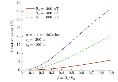
Fig. 5. Relative errors vary with Bc/B0 under different conditions of amplitudes of the actual magnetic fields Bx.
4.2. The n=–2 modulation for different amplitudes of the carrier magnetic field
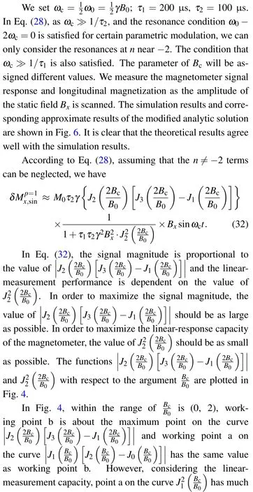
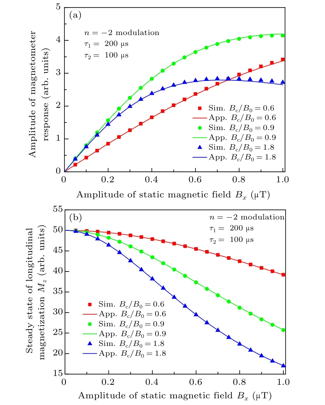
Fig.6. Magnetometer output for n=−2 modulation under different conditions of amplitudes of the carrier magnetic field: (a) the amplitude of magnetometer response; (b) the steady state of longitudinal magnetization Mz. “Sim.” and“App.” in the figure denote numerical simulation and approximate analytical results,respectively.
4.3. The n = –1 modulation for different longitudinal and transverse relaxation time
Setting ωc=ω0=γB0;Bc/B0=1.5;the parameters of τ1and τ2will be assigned different values and the condition that ωc≫1/τ1, ωc≫1/τ2should be satisfied for all examples.We measure the magnetometer signal response and longitudinal magnetization as the amplitude of the static field Bxis scanned.
The simulation results and corresponding approximate results of the modified analytic solution are shown in Fig.7. It is clear that the theoretical results agree well with the simulation results.According to Eq.(30)and Fig.7,it can be seen that the smaller the spin relaxation time,the smaller the signal magnitude but the higher the linear-measurement capacity. When choosing proper parameters for the carrier magnetic fields and spin relaxation time, we should consider the fact that Bcwill also influence the spin relaxation.[19]Furthermore,if the precise values of τ2and other working conditions are known,we can obtain the value of τ1by fitting the magnetometer response curve with our modified theoretical model, which provides a new method to measure the longitudinal spin relaxation time τ1.

Fig.7. Magnetometer output for n=−1 modulation under different conditions of longitudinal and transverse relaxation time: (a) the amplitude of magnetometer response; (b) the steady state of longitudinal magnetization Mz. “Sim.” and“App.” in the figure denote numerical simulation and approximate analytical results,respectively.
4.4. The n=–1 modulation for different angular frequency of the rotation field
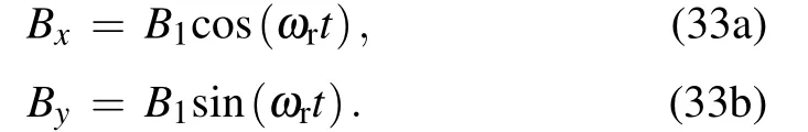
As already noted in the beginning, NMR detection in a spin-exchange NMR oscillator can be realized by using the alkali atoms as an integrated magnetometer.In NMR oscillators,by applying a“drive”field that rotates in the same direction as the nuclear spins and at a frequency close to their NMR frequency,the nuclear spins can be induced to precess about the z-axis. Assuming that B1rotates about the z-axis with amplitude B1and angular frequency ωr, the components of the rotation field along x-axis and y-axis are
Then, a rotating coordinate system x′y′z is introduced to simplify the analysis,as shown in Fig.8. The rotating coordinates are defined by the condition that x′-axis rotates in phase with B1about the z-axis and y′-axis rotates in quadrature. The rotation field is the equivalent of a static field in the rotating coordinate system.
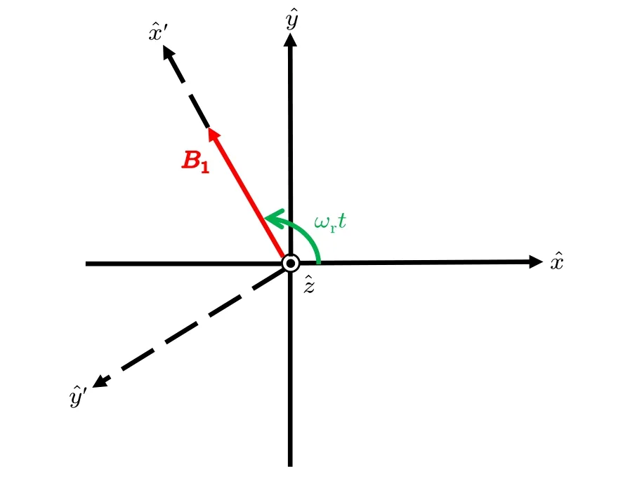
Fig.8. xyz: laboratory coordinate system and x′y′z: rotating coordinate system.
Therefore,we have the relations

Substituting Eqs.(33a)and(33b)into Bloch-like Eq.(1),and using Eqs. (34a) and (34b), the following equations are obtained in the rotating coordinate frame:

where M+′=Mx′+iMy′.
Comparing Eqs. (35a) and (35b) and Eqs. (2a) and (2b),using the same method to derive the solutions to Eqs.(2a)and(2b),we can obtain the solutions to Eqs.(35a)and(35b).Considering the quadrature demodulation at harmonic pωc, we have

where
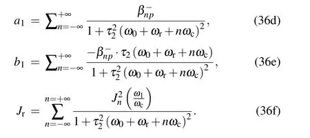
According to Eq.(34a),we can obtain the magnetometer signal
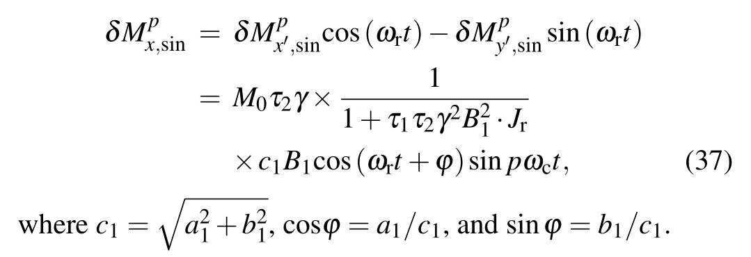
Equation (37) shows that the angular frequency ωrnot only influences the amplitude-frequency response,[20]but the linear-measurement characteristics of the magnetometer when measuring the rotation field.
Then, we conduct the simulation experiments to verify the modified analytical model of Eq. (37). We consider the first (p = 1) harmonics of the modulation and observe the n=−1 modulation,ωc=ω0=γB0,and we set Bc/B0=1.5,τ1=200 µs, τ2=100 µs. As ωr≪ωc, ωc≫1/τ2, we can only consider the resonances at n near −1. The condition that ωc≫1/τ1is also satisfied. The parameter of ωrwill be assigned different values. We measure the magnetometer signal response and longitudinal magnetization as the amplitude of the rotation field B1is scanned. The simulation results and corresponding approximate results of the modified analytical solution are shown in Fig. 9. It is clear that the theoretical results agree well with the simulation results.
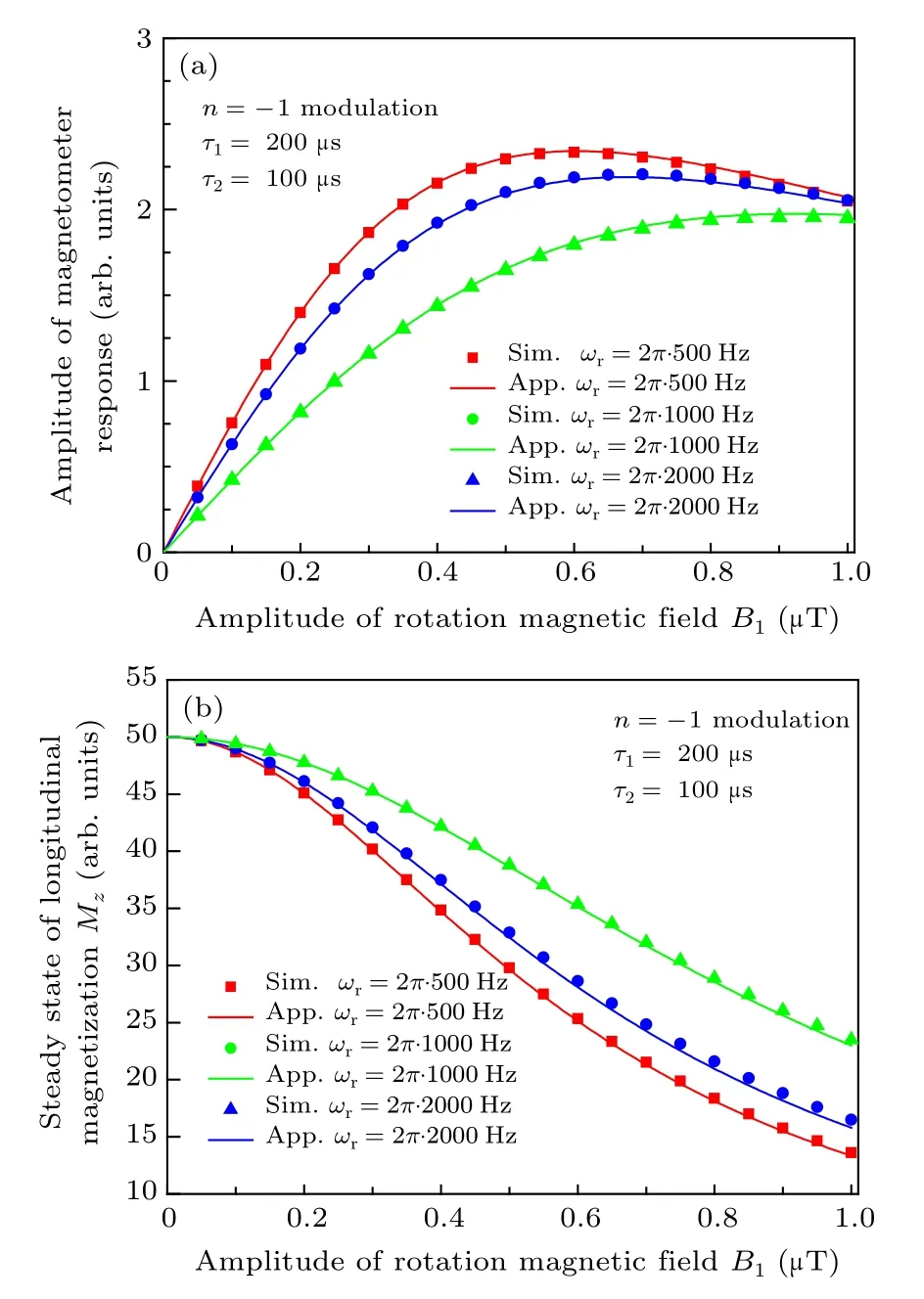
Fig.9. Magnetometer output for n=−1 modulation under different conditions of angular frequency of the rotation field: (a) the amplitude of magnetometer response; (b) the steady state of longitudinal magnetization Mz. “Sim.” and“App.” in the figure denote numerical simulation and approximate analytical results,respectively.

Combining Eq. (38) and Fig. 9, it can be clearly seen that the higher the angular frequency ωrof the rotation field,the smaller the signal magnitude but the higher the linearmeasurement capacity of the magnetometer.
5. Conclusion
In summary,for the AMA magnetometer employing longitudinal carrier field, the amplitude of the magnetometer response is not proportional to the measured magnetic fields Bxwhen Bxis large, because the longitudinal magnetization Mzwill be influenced by and vary with Bx. By theoretical derivation using the perturbation-iteration method,we present a modified theoretical model to more definitely analyze the practical linear-response characteristics of the magnetometer,which are determined by different working conditions. For the amplitude Bcand frequency ωcof the carrier field, the spin relaxation time τ1and τ2, and the rotation frequency ωrof the measured transverse fields, the smaller the values of|Jn(nBc/B0)|(when ωc=ω0/n)and τ1τ2,and the higher the rotation frequency ωr,leading to higher linear-response capacity of the magnetometer. The larger amplitudes of the actual magnetic fields Bxto be measured,the larger the measurement error based on the existing fundamental model.
Hence, we can use this modified model to modify the measurement results to obtain more accurate values of the actual Bxand to optimize the working conditions and choose proper system parameters to achieve the desired performance for practical magnetometer systems. This modified theoretical model to describe the linear-response curves also provides a new method to measure the longitudinal relaxation time τ1for the alkali metal magnetometer.

- Chinese Physics B的其它文章
- Corrosion behavior of high-level waste container materials Ti and Ti–Pd alloy under long-term gamma irradiation in Beishan groundwater*
- Degradation of β-Ga2O3 Schottky barrier diode under swift heavy ion irradiation*
- Influence of temperature and alloying elements on the threshold displacement energies in concentrated Ni–Fe–Cr alloys*
- Cathodic shift of onset potential on TiO2 nanorod arrays with significantly enhanced visible light photoactivity via nitrogen/cobalt co-implantation*
- Review on ionization and quenching mechanisms of Trichel pulse*
- Thermally induced band hybridization in bilayer-bilayer MoS2/WS2 heterostructure∗