Effects of Time-varying Delays on the Stability of a Class of Stochastic Competitive System

ZHAO Jinxing(赵金星)，SHAO Yuanfu(邵远夫)

(1.School of Mathematical Sciences，Inner Mongolia University，Hohhot 010021，China;2.College of Science，Guilin University of Technology，Guilin 541004，China)

Abstract:A class of stochastic competitive system with time-varying delays is proposed in this paper.By use of the theory of neutral differential equation and constructing suitable functional，we are concerned with the globally asymptotical stability and stability in probability of the equilibrium state.Finally，some numerical simulations are given to validate our main results.

Key words:Time-varying delay;Equilibrium state;Asymptotical stability;Stability in probability

1.Introduction

For biological system，the existence and stability of equilibrium point or periodic solution is very valuable for people to understand and control dynamic system，which is basic and the most important dynamical behavior.Many researchers have obtained many nice results.[1－4]

In general，time delays usually appear in population system[5－6].There are many kinds of time delays，such as constant delays[6]，distributed delays[7－8]and time-varying delays[9－10，17].For example，LIU[17]proposed a two-species competitive system with time-varying delays as follows:

For the deterministic system(1.1)，let

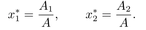
For the latter study，we assume that(1.1)has a unique positive equilibrium point as follows:

On the other hand，population system is often subject to environmental fluctuation，and hence，it is necessary to consider stochastic effects in the process of mathematical modeling[11－18].Many stochastic systems have been investigated，such as stochastic competitive system[11]，stochastic cooperative system[12].Meanwhile，time delays often appear and bring important influence to the dynamics of stochastic systems[13－18].

In real world，stochastic perturbations are complex and presented as many forms.For example，the authors[11，13]show that，stochastic perturbations of the state variables around their steady-state are of Brownian white noise，which are proportional to the distance ofx1，x2from the equilibrium statex*=()Trespectively.Consequently，we firstly propose the following stochastic competitive system with time-varying delays:

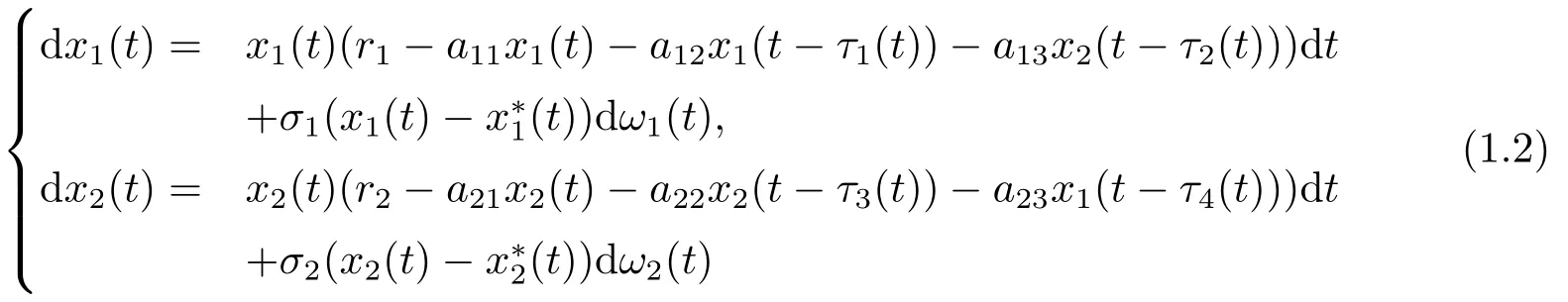
with initial data

wherexi(t)stands for the population size of theith species at timet，ri＞0 is the growth rate ofxi(t).Parametersa11，a12，a21，a22are positive and represent the intra-specific competitive coefficient，anda13＞0，a23＞0 are the interspecific competitive rates ofx1(t)andx2(t)，respectively.τj(t)＞0 is time-varying delay，is positive and continuous function defined on[-τ，0];denotes the intensity of white noise，ωi(t)t＞0is the standard independent Brownian motion defined on a complete probability space(Ω，F，Ft≥0，P)，i=1，2.

Further，stochastic perturbations of state variables are proportional to the product ofx1，x2and their distance from equilibrium stateandwhich may refer to[14，17].Considering this kind of stochastic influence，we have the following stochastic model with timevarying delays proposed by LIU[17].

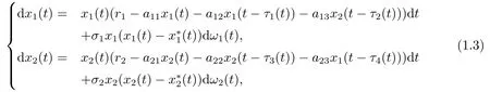
where the meanings of all parameters are as before.

In view of the importance of equilibrium state for dynamical system，in this paper，our main aim is to investigate the effect of time delays on the equilibrium state of(1.2)and(1.3)，respectively.

The rest work of this paper is organized as follows.In Section 2，we give some definitions，notations and some important lemmas.Section 3 focuses on the main results such as global attactivity and the stability in probability.Some numerical examples are given in Section 4 to validate our theoretical results.Finally a brief conclusion and discussion are given in Section 5 to conclude the paper.

2.Preliminaries

Let{Ω，σ，P}be a probability space，{ft，t≥0}be a family ofσ-algebras，ft∈σ.Consider the following neutral stochastic differential equation:

whereHis the space off0-adapted functionsφ(s)∈Rn，s≤0 andxt(s)=x(t+s)，s≤0，ω(t)ism-dimensionalft-adapted Brownian process，a(t，φ)，b(t，φ)aren-dimensional vector andn×m-dimensional matrix，respectively.Define||φ||0=sups≤0|φ(s)|，and||φ||1=sups≤0E{|φ(s)|2}，where E denotes the mathematical expectation.

Definition 2.1The zero solution of(2.1)is said to be stable in probability if for anyϵ，ε＞0，there exists a numberδ＞0 and the solutionx(t)=x(t，φ)such thatP{|x(t，φ)|＞ϵ}＜εfor any initial functionφ∈HsatisfyingP{||φ0||≤δ}=1，wherePis the probability of an event.

Lemma 2.1Systems(1.2)and(1.3)have a unique global positive solution ont＞-τfor any initial data given above，respectively.

Remark 2.1The proof is very standard and is omitted here.Readers may refer to[17].

Lemma 2.2[19]If there exists a functionalV(t，x)such that

for any functionφ∈HsatisfyingP{||φ||0≤δ}=1，andδ＞0 is sufficiently small positive constant，then the zero solution of(2.1)is stable in probability.

For the latter discussion，we give a technical assumption.

Assumption 2.1Assume the derivatives of all delays satisfy the following condition:

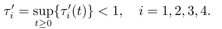
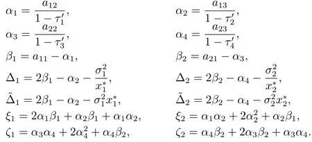
For simplicity，we denotef(t)byfand apply the following notations in the later.

3.Delay Effects on The Equilibrium State

In this section，we study the time delay effects on the dynamical behaviors of the equilibrium state of(1.2).Lety1(t)=x1(t)2(t)=x2(t)then(1.2)is transformed to the following equivalent system:

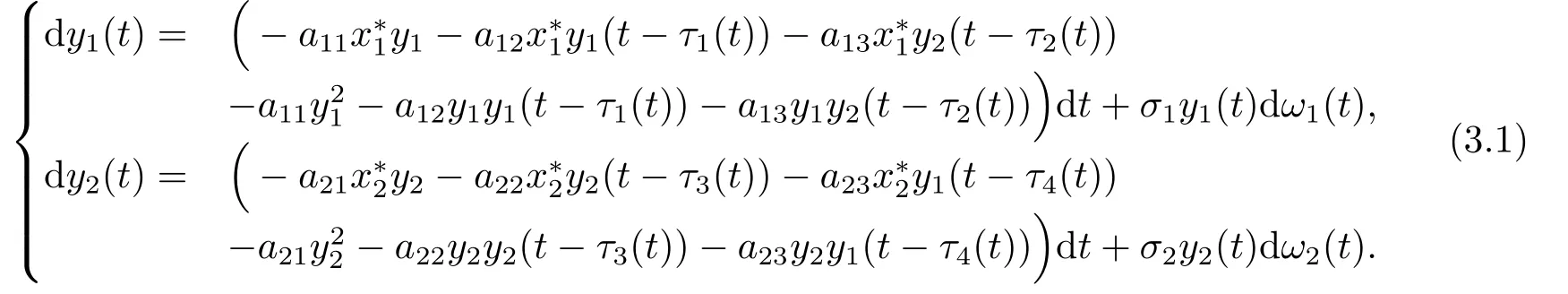
By transformation，the stability of equilibrate state of(1.2)is equivalent to the stability of zero solution of(3.1).Consequently，in order to study the stability of the equilibrate state of(1.2)，we only need to study the stability of zero solution of(3.1).

By use of the definition of derivative，we have

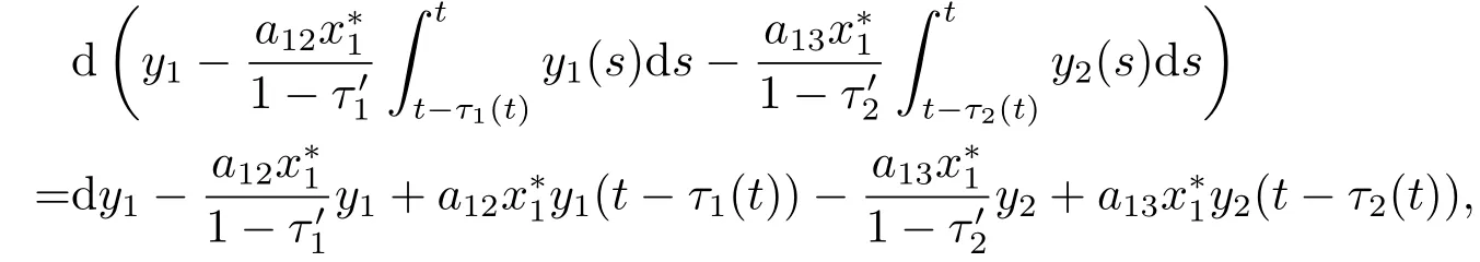
and

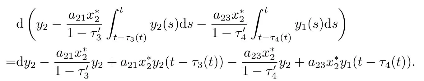
Therefore，(3.1)is equivalent to the following system.

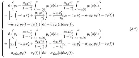
Firstly，we consider the linear case of(3.2)as follows.

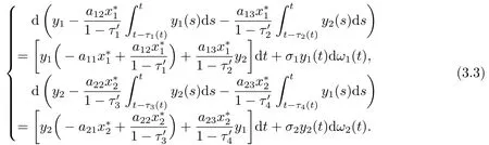
For the system(3.3)，we have the following result.

Assumption 3.1

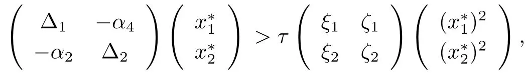
where the matrixC=(cij)＞B=(bij)meanscij＞bijfor anyi=1，···，n，j=1，···，m.

Theorem 3.1If Assumption 3.1 holds，then the zero solution of(3.3)is globally asymptotically stable，almost surely.

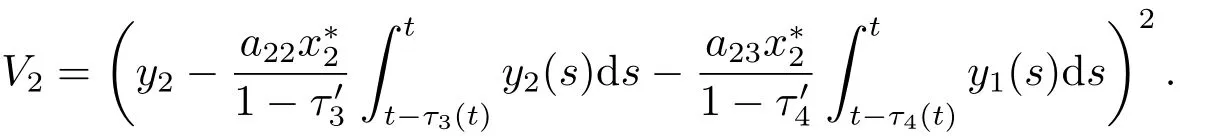
ProofFirstly，we define two functions as follows:

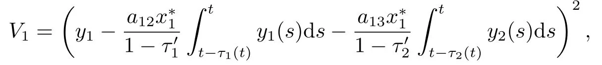
and

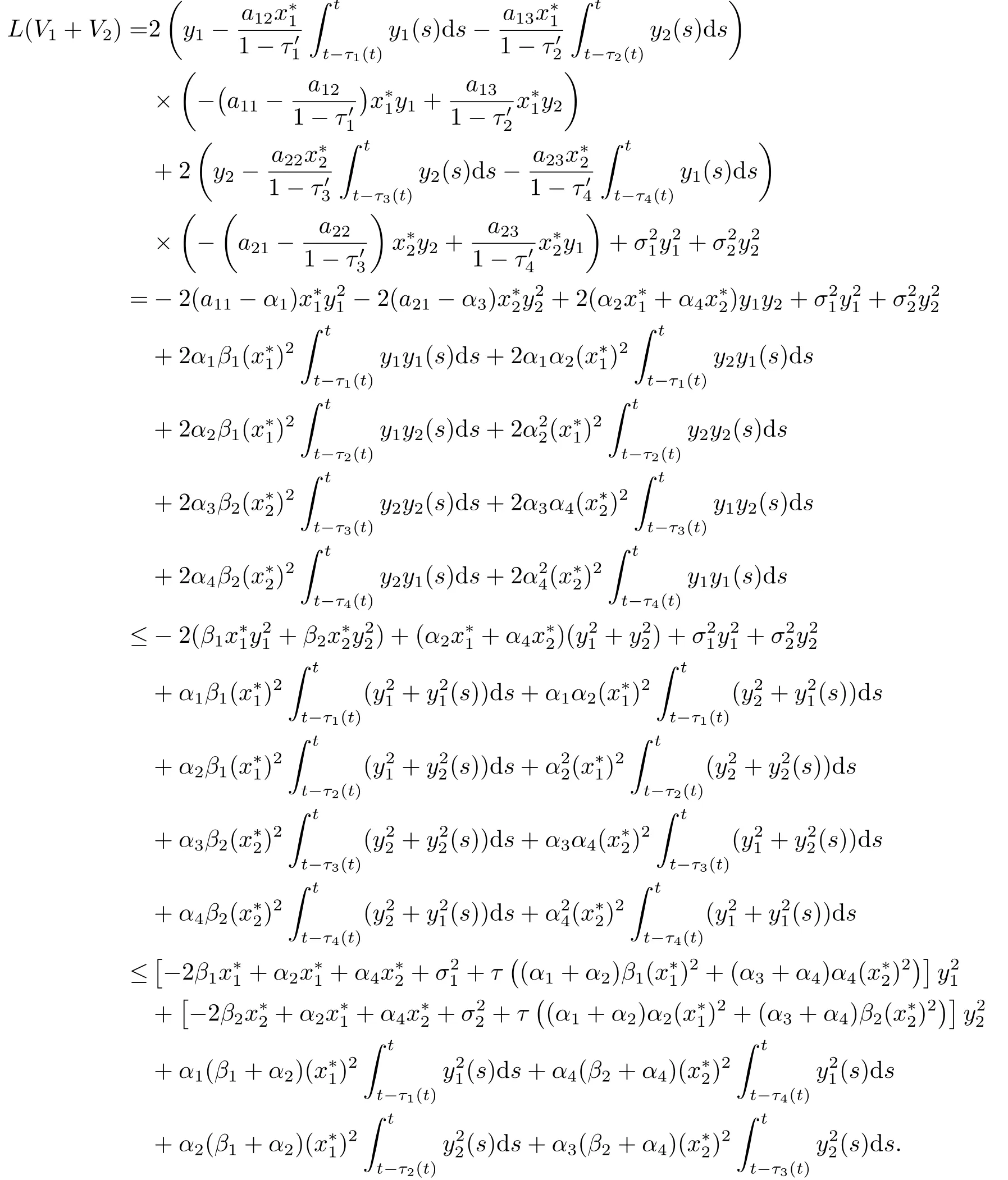
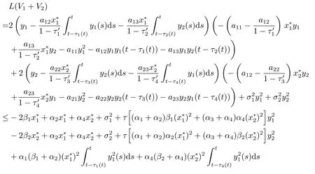
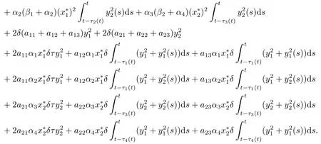
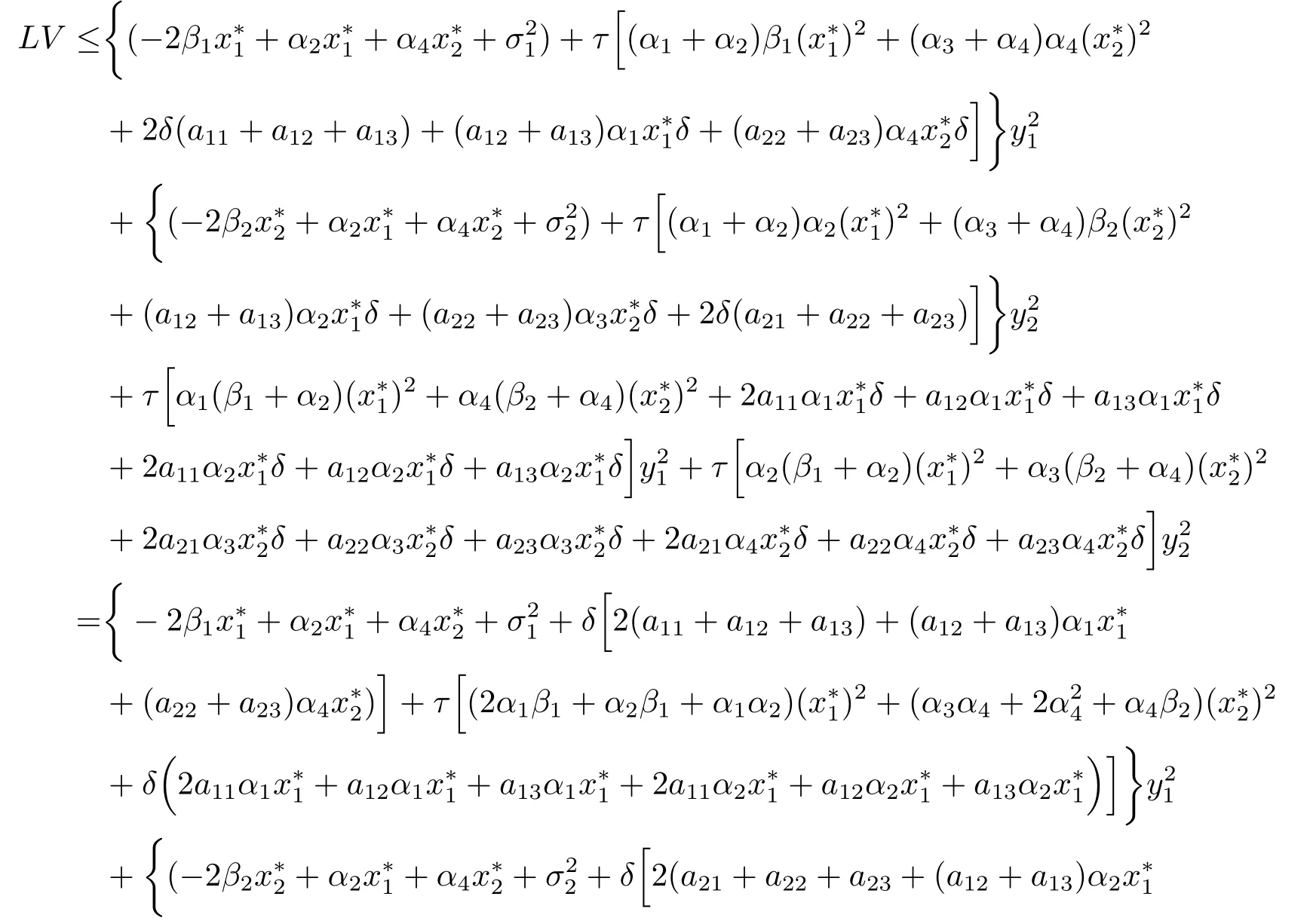
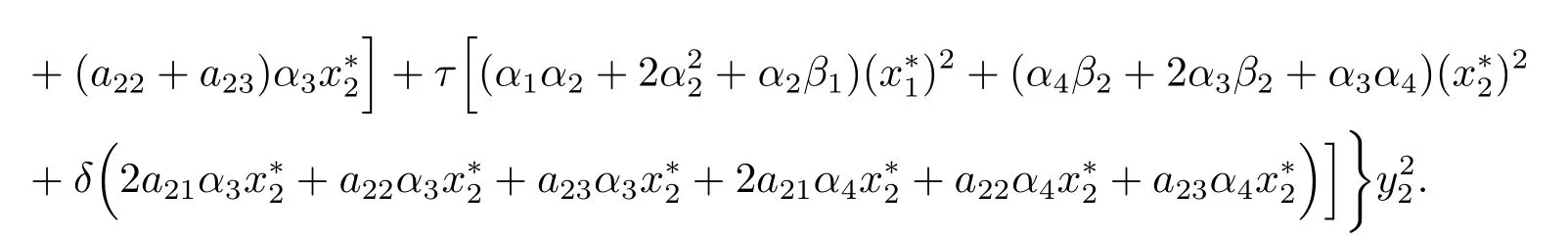
Applying the itˆo formula toV1andV2，we have

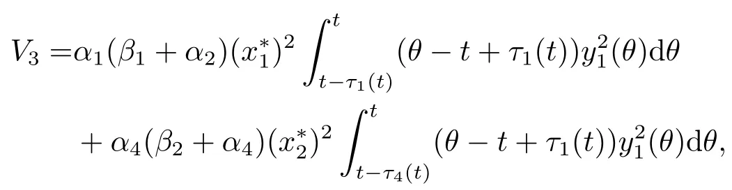
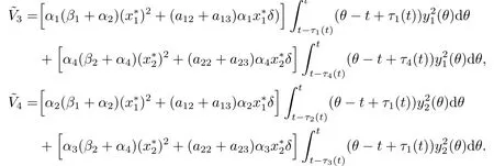
Define

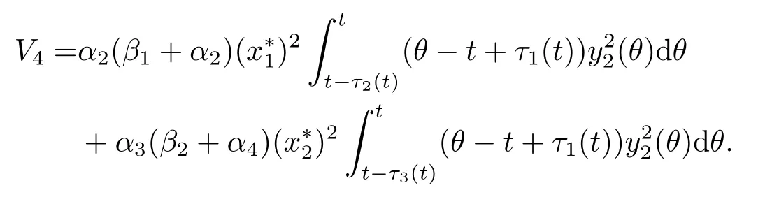
and

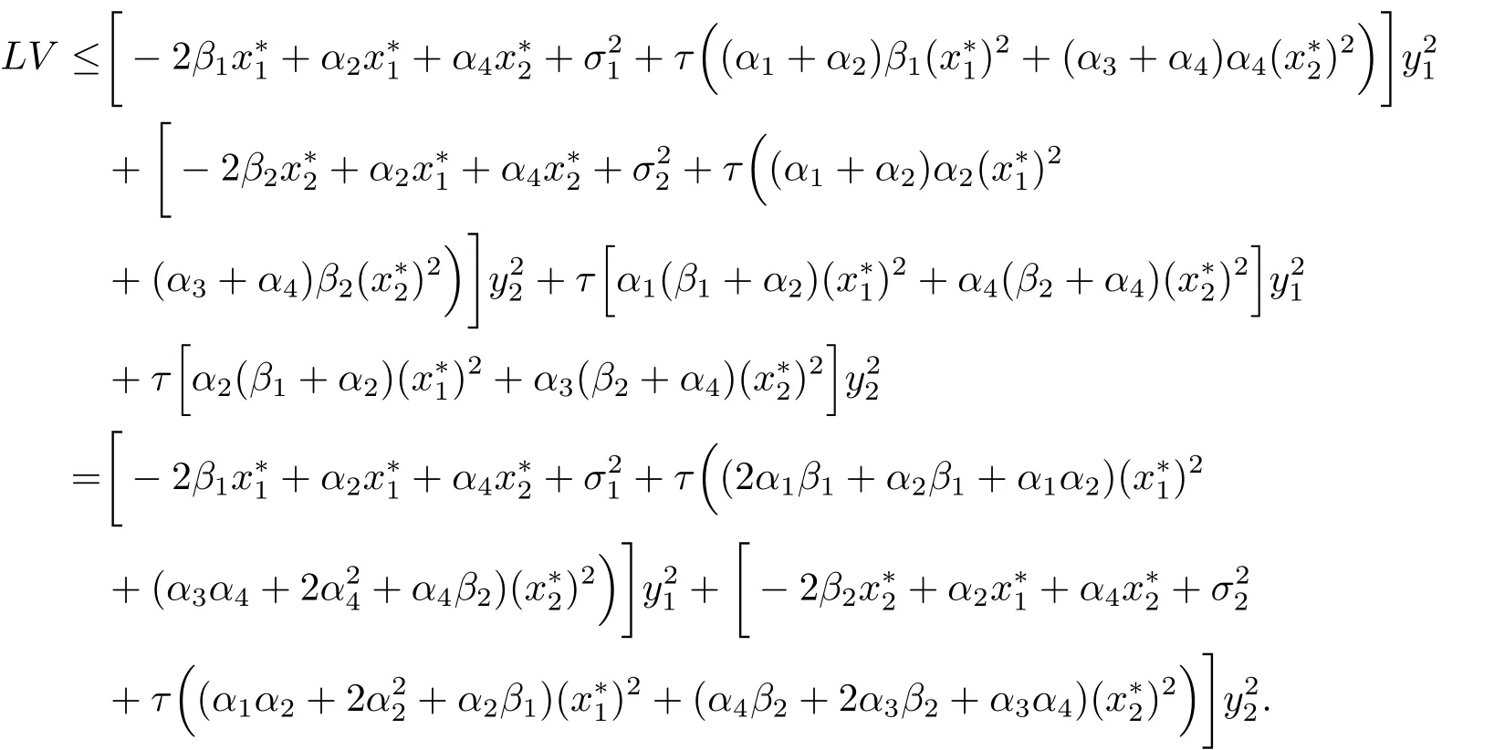
Clearly，using Assumption 3.1，we haveLV＜0 along all trajectories inexcept the equilibrium state.Hence，by the stability theory of stochastic functional differential equations，the zero solution of(3.3)is globally asymptotically stable.This completes the proof.

Theorem 3.2If Assumption 3.1 holds，then the zero solution of system(3.2)is stable in probability，that is，the equilibrium state of(1.2)is stable in probability.

ProofFor the system(3.2)，we define the same functionsV1，V2as before.We assume that there exists a numberδ＞0 such that supt≥τ|xi(s)|＜δ，i=1，2.Using the itˆo formula and calculatingLV1，LV2along the system(3.2)respectively，we obtain

Define

By choosing sufficiently smallδ＞0 satisfying Assumption 3.1，thenLV＜0 holds.Therefore，by Lemma 2.2，the zero solution of(3.2)is stable in probability.The proof is completed.

Next we begin the process of investigating the stability of system(1.3).Lety1(t)=Then(1.3)is transformed to the following equivalent system.

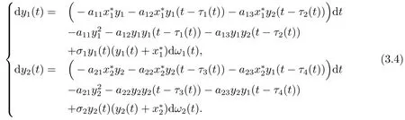
Consequently，the stability of equilibrate state of(1.3)is equivalent to the stability of zero solution of(3.4).By transformation，(3.4)is equivalent to the following system:

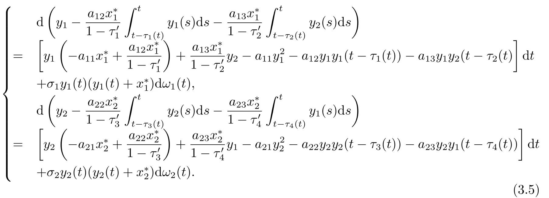
We consider the following linear case of(3.5).

Assumption 3.2

Theorem 3.3If Assumption 3.2 holds，then the equilibrium state of(3.5)is stable in probability，i.e.，the equilibrium state of(1.3)is stable in probability.

ProofDefine two same functionalsV1，V2as before，using Itˆo’s formula and computingLValong(3.6)，we have

The rest of the proof is similar to Theorem 3.1 and Theorem 3.2，hence we omit it here.

Remark 3.1System(1.3)was considered in[17].By constructing some functionals，the author discussed the global attractivity of equilibrium point.Similarly，we discuss the global attractivity of(1.3)，but the method applied here is by constructing an neutral differential equation to get the suitable functional，which is very different from[17].Moreover，our result is related to the equilibrium state and presents the effects of time-varying delays on the dynamical behaviors of(1.3)，which is also different from[17].On the other hand，we also establish the sufficient conditions of making equilibrium state keeping stable in probability，which is not discussed in[17].As the special case of(1.3)，ifτ=0，we show the differences between Theorem 3.3 and Theorem 1 in[17]by giving a numerical example in the next section(see Fig.4.7).

4.Numerical Simulations

In this section，some numerical examples are given to verify our theoretical results.By applying the Milstein method[20]and writing Matlab codes，we give some numerical results as follows.

Leta11=1.8，a12=0.5，a13=0.3，a21=1.5，a22=0.3，a23=0.5，r1=2，r2=2.5，τ1(t)=An easy computation yieldsA=3.99，A1=2.85，A2=4.75=0.7143=1.1905=1/5=2/5=2/5=a11-α1=1.175，β2=a21-α3=1.

Ifσ1=0.6，σ2=0.6，τ=0.04，thenΔ1=1.646，Δ2=1.0309，=1.8929，=0.9047，ξ1=2.3687，ξ2=1.4，ζ1=1.889，ζ2=2，and

By verification，Assumption 3.1 holds，and hence，Theorem 3.1 and Theorem 3.2 imply that the system(1.2)is globally attractive and stable in probability(see Fig.4.1).

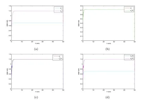
Fig.4.1 Time series of x1(t)and x2(t)of(1.2)with σ1=0.6，σ2=0.6，τ=0.04.(a)Equilibrium point of system(1.2)，(b)Time series of x1(t)and ，(c)Time series of x2(t)and x*2，(d)time series of x1(t)and x2(t)

Ifσ1=3，σ2=6 and other parameters keep unchanged，then Assumption 3.1 does not hold，hence the system(1.2)may be unstable(see Fig.4.2).

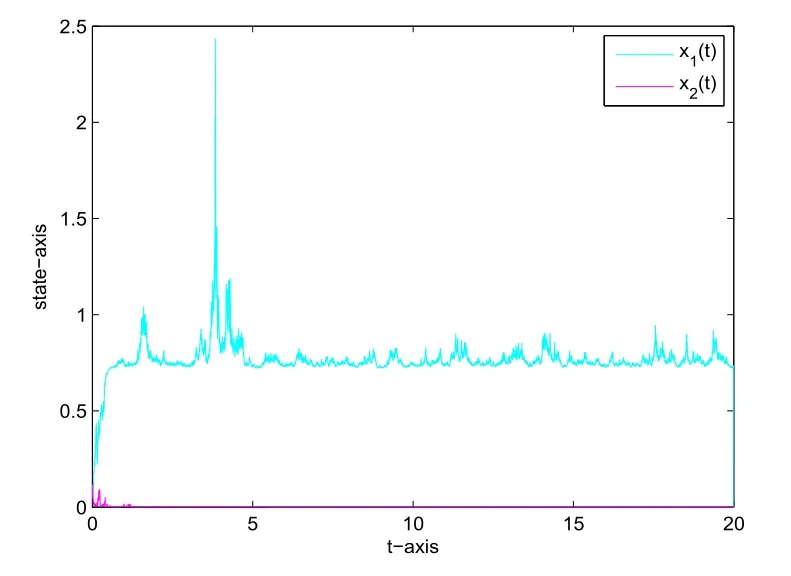
Fig.4.2 Time series of x1(t)and x2(t)of(1.2)with σ1=3，σ2=6，τ=0.04，which shows x2 is extinct and the system is unstable

Similarly，if other parameters are as before andτ=8，then Assumption 3.1 does not hold and the system(1.2)may be also unstable(see Fig.4.3).

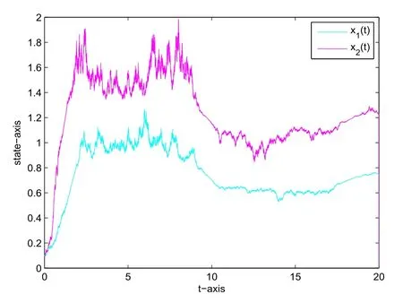
Fig.4.3 Time series of x1(t)and x2(t)of(1.2)with σ1=0.6，σ2=0.6，τ=8，which shows species x1(t)and x2(t)are unstable

For the system(1.3)，ifσ1=0.6，σ2=0.6，τ=0.04，and other parameters are as before.By verification，Assumption 3.2 holds and(1.3)is stable(see Fig.4.4).

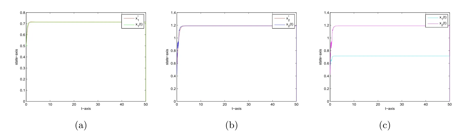
Fig.4.4 Time series of x1(t)and x2(t)of(1.3)with σ1=0.6，σ2=0.6，τ=0.04.(a)Time series of x1(t)and ，(b)Time series of x2(t)and (c)Time series of x1(t)and x2(t)

Ifσ1=6，σ2=6，τ=0.04，orσ1=0.6，σ2=0.6，τ=8，and other parameters keep unchanged，then Assumption 3.2 does not hold，and the system(1.3)may be unstable(see Fig.4.5 and Fig.4.6，respectively).

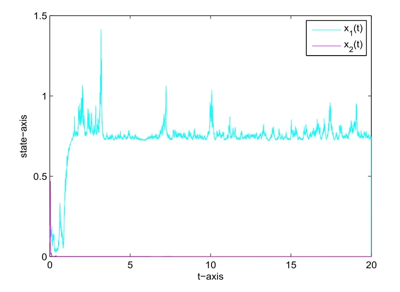
Fig.4.5 Time series of x1(t)and x2(t)of(1.3)with σ1=3，σ2=6，τ=0.04，which shows x2 is extinct and the system is unstable

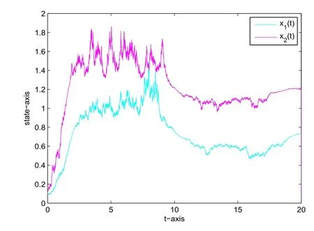
Fig.4.6 Time series of x1(t)and x2(t)of(1.3)with σ1=0.6，σ2=0.6，τ=8，which shows species x1(t)and x2(t)are unstable

If there is no delays，i.e.，=0，τ=0(i=1，2，3，4).Seta11=0.9，a12=0.6，a13=0.3，a21=0.8，a22=0.5，a23=0.3，r1=1，r2=1，σ1=σ2=0.9，then=0.5376=0.6452.By computation，the conditions of Theorem 1 in[24]do not hold，hence we can not obtain the global attarctivity.But it is clear that

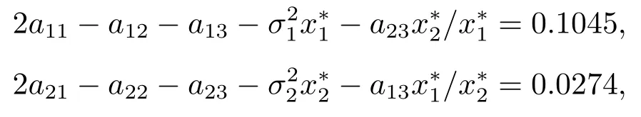
which meets the condition of Theorem 3.3，therefore，the system is globally attractive and stable in probability，which is illustrated in Fig.4.7.

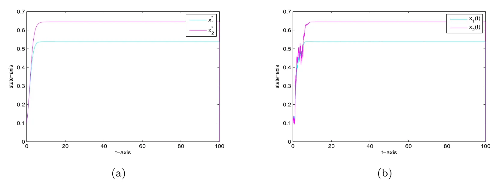
Fig.4.7 Time series of x1(t)and x2(t)of(1.3)with σ1=0.6，σ2=0.6，τ=0.(a)Equilibrium points of system(1.3)without delays，(b)Time series of x1(t)and x2(t)without delays

5.Conclusion and Discussion

In this paper，we consider a class of stochastic competitive system with time-varying delays.Theorem 3.1 gives the sufficient conditions assuring the global stability of the equilibrium state.Theorem 3.2 and Theorem 3.3 show that under some conditions，the equilibrium state of(1.2)and(1.3)are stable in probability，respectively.Our obtained results show that time-varying delays have some significant effects on the globally asymptotic stability of positive equilibrium state.Whereas in practice，multi-species system often appears and exhibits more complex dynamical behaviors.For multi-species system，we believe that there may be some similar results，which is interesting and left for our work in the future.