A DIFFUSIVE SVEIR EPIDEMIC MODEL WITH TIME DELAY AND GENERAL INCIDENCE∗

(周金玲)Xinsheng MA (马新生)

Department of Mathematics,Zhejiang International Studies University,Hangzhou 310023,China E-mail:jlzhou@amss.ac.cn;xsma@zisu.edu.cn

Yu YANG (杨瑜)†

School of Statistics and Mathematics,Shanghai Lixin University of Accounting and Finance,Shanghai 201209,China E-mail:yangyu@lixin.edu.cn

Tonghua ZHANG (张同华)

Department of Mathematics,Swinburne University of Technology,Hawthorn,Victoria 3122,Australia E-mail:tonghuazhang@swin.edu.au

Abstract In this paper,we consider a delayed diffusive SVEIR model with general incidence.We first establish the threshold dynamics of this model.Using a Nonstandard Finite Difference(NSFD)scheme,we then give the discretization of the continuous model.Applying Lyapunov functions,global stability of the equilibria are established.Numerical simulations are presented to validate the obtained results.The prolonged time delay can lead to the elimination of the infectiousness.

Key words SVEIR model;vaccination;Lyapunov function;nonstandard finite difference method

1 Introduction

Vaccination is an effective way of controlling the transmission of infectious diseases such as tuberculosis and tetanus etc..Thus,many countries provide routine vaccination against all of these diseases.However,vaccine-induced immunity may wane as time goes on.To better understand this phenomenon,mathematical models have been developed.Kribs-Zaleta and Velasco-Hernndez[1]considered an SIS disease model with vaccination.Arino et al.[2]investigated an SIRS model with vaccination.Li et al.[3]indicated that vaccine effectiveness plays a key role in disease prevention and control.To describe vaccination strategy,Liu et al.[4]considered SVIR epidemic models.LetS,V,IandRbe the susceptible,vaccinated,infectious and recovered individuals,respectively.Furthermore,Li and Yang[5]proposed the following model fort>0:

HereµandArepresent the death rate and the birth rate,respectively.q<1 denotes the fraction of the vaccinated newborns,pis the unvaccinated newborns,0<σ<1 represents that the vaccine is not completely effective,βis the transmission coefficient of the susceptible,γis the recovery rate,δis the per capita disease-induced death rate.The susceptible population is vaccinated at a constant rateαand the vaccine-induced immunity wanes at rateη.Li and Yang discussed the global dynamics of system(1.1)by applying Lyapunov functions.

As seen from the existing models,incidence rates play a very important role in determining model dynamics;for example,the bilinear incidence rate is applicable to Hand-Foot-and-Mouth disease[6],H5N1[7]andSARS[8],but not to sexually transmitted diseases[9].To model the effect of behavioural changes,Liuetal.[10]proposed an incidence rate.Tomodelthe cholera epidemics in Bari,Capasso and Serio[11]considered the incidence ratep=q=1.Due to a diseases latency,or factors of immunity,infection processes are not instantaneous.Hence,time delay is important in studying infectious disease dynamics.Hattaf et al.[12]studied a delayed SIR model with general incidence.Wang et al.[13]proposed a delayed SVEIR model with nonlinear incidence.Recently,Hattaf[14]proposed a generalized viral infection model with multi-delays and humoral immunity.For more works on delayed epidemic models with vaccination,we refer readers to[15–19].

All of the above mentioned works are location independent,but location-dependent phenomenon are not uncommon in mathematical biology(see[20–22]).Webby[23]pointed out that infectious cases can first be found at one location and can then spread to other areas.Therefore,it is interesting to study epidemic models with spatial diffusion.Xu and Ai[24]considered an in fluenza disease model with spatial diffusion and vaccination.Abdelmalek and Bendoukha[25]proposed a diffusive SVIR epidemic model allowing continuous immigration of all classes of individuals.Xu et al.[26]discussed a vaccination model with spatial diffusion and nonlinear incidence.

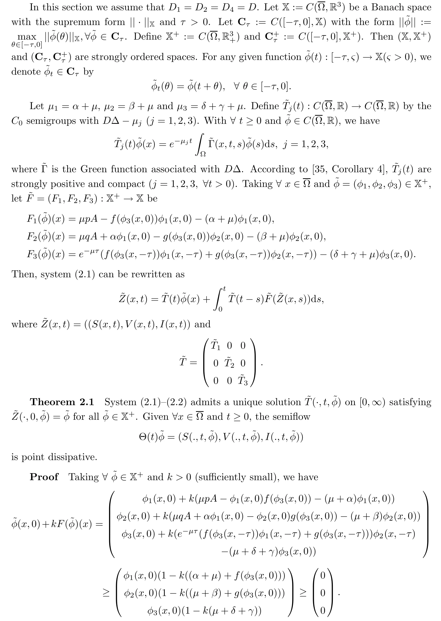
Let Ω be a bounded domain in Rnwith smooth boundary∂Ω.LetDi(i=1,2,3,4,5)be the diffusion rate and∆be the Laplace operator.Then,motivated by the aforementioned works,particularly[13,23],we study the delayed SVEIR model with spatial diffusion as follows:

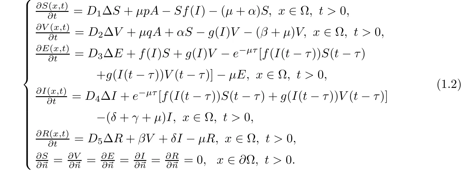
Here,τrepresents the latent period of the disease.The other parameters are as described for system(1.1).Denote by→nthe outward unit normal vector of∂Ω as in[20,21].We further consider model(1.2)with initial condition

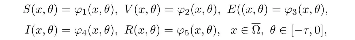
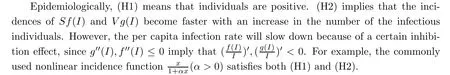
whereϕi(i=1,2,3,4,5)are uniformly continuous and bounded.Functionsgandfsatisfyg(0)=f(0)=0 and

(H1)forI>0,g(I)>0 andf(I)>0;

(H2)forI≥0,g′(I)>0 andf′(I)>0,g′′(I)≤0 andf′′(I)≤0.

In this study,in addition to model(1.2),we will also investigate the discrete analogue,due to the fact that epidemiological data is usually collected daily,monthly,or even yearly,but not continuously.Hence,it is more reasonable to use a discrete model to study the transmission mechanism of infectious disease.Furthermore,it is an interesting problem as to whether or not a selected difference scheme can preserve the positivity,boundedness and global stability for the corresponding continuous model.In this regard,some researchers have applied the NSFD scheme proposed by Mickens[27]to discuss the dynamical behaviors of different epidemic models([28–37]).

The rest of the paper is organized as follows:in Section 2,we establish the global dynamics of the continuous model(1.2).In Section 3,we derive the discretization of(1.2)by the NSFD scheme and establish the positivity and boundedness of the solution.By using discrete Lyapunov functionals,we discuss the global stability of the equilibria of the discretised model in Section 4.This is then followed by numerical simulations in Section 5 to illustrate the obtained results.

2 The Continuous Model

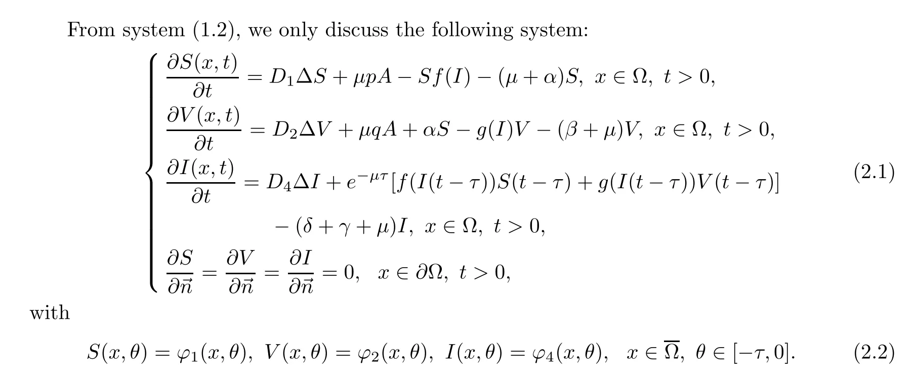
2.1 Threshold dynamics

The above inequality implies that

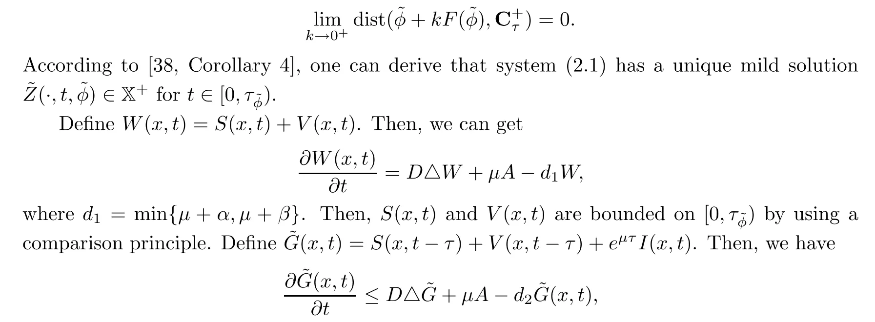
whered2=min{µ,µ+β,µ+δ+γ}.Thus,(x,t)are bounded on[0,τφ˜),by the comparison principle.This implies thatI(x,t)are also bounded on[0,τφ˜).The remaining proofs are similar to Theorem 2.1 of Zhou et al.[34],which we omit here.

2.2 Existence of equilibria

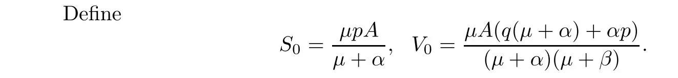
Then,E0(S0,V0,0)is the disease-free equilibrium of system(2.1).The basic reproduction number is

The endemic equilibrium should satisfy

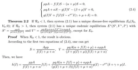
Obviously,h(+∞)=−∞andh(0)=0.It follows fromh′(0)>0 thath(I)=0 has at least one positive solution denoted byI∗,where

This is equivalent to R0>1.Thus,(2.4)has at least one positive solution with

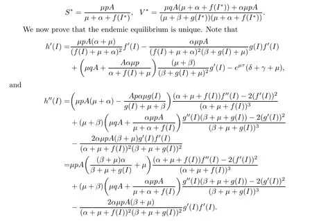
By(H2),we know thath′′(I)<0 forI>0.If there exists more than one positive equilibrium,then there must exist a pointE∗(S∗,V∗,I∗)such thath′′(I∗)=0.We obtain a contradiction.

2.3 Local stability

Let 0=µ0<µi<µi+1be the eigenvalues of−∆on Ω,andE(µi)be the space of eigenfunctions withµi(i=1,2...).Then,we de fine the orthonormal basis ofE(µi)(i=1,2...)by{φij:j=1,2,...,dimE(µi)}as follows:

Here,Xij={cφij:c∈R3}.In a fashion similar to[20,Theorem 3.1],one gets the following result:

Theorem 2.3If R0<1,thenE0of system(2.1)is locally asymptotically stable.

ProofLinearizing system(2.1)atE0,we get

Clearly,(2.5)has eigenvaluesλ1=−(µiD+µ+α)<0 andλ2=−(µiD+µ+β)<0.The other eigenvalueλ3satis fies

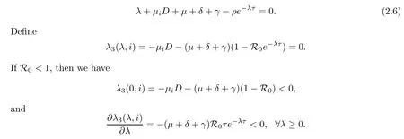
Thus,(2.6)has no positive real root.

Assume that(2.6)has a complex rootλ=ω1+iω2withω1≥0;substituting it into(2.6),one has

Squaring and adding these equations together,we obtain

Usingω1≥0 andµi≥0,we have

when R0<1.This is a contradiction.Therefore,(2.6)has no complex root with a non-negative real part.Consideringi=0 and the space X0corresponding toµ0=0,we get

when R0>1.Therefore,there exists a constantλ0>0 such thatλ3(λ0,0)=0,yielding that(2.6)has at least one positive root.

2.4 Global stability

De fine Φ(x)=x−1−lnx.It is clear that Φ(x)≥0 for allx>0.It follows from(H2)thatg′(I)is nonincreasing,so one can obtaing(I)=g(I)−g(0)=g′(η)(I−0)≤g′(0)I,whereηis between 0 andI.Similarly,one hasf(I)≤f′(0)I.

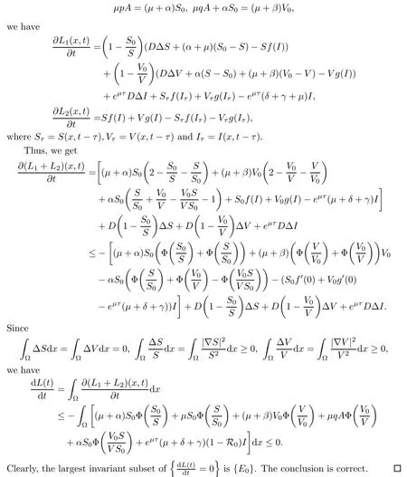
Theorem 2.4If R0≤1,thenE0of system(2.1)is globally asymptotically stable.

ProofDe fine

According to lnx≤x−1 and

Theorem 2.5If R0>1,thenE∗of system(2.1)is globally asymptotically stable.

ProofDe fine

In a manner similar to the proof of Theorem 2.4,the conclusion is proved.

3 A Discretized Model

The equilibria of system(3.1)is the same as for(2.1).Applying M-matrix theory[39],we have the following result:

Theorem 3.1For any△x>0 and∆t>0,the solution of system(3.1)with(3.2)and(3.3)is nonnegative and bounded.

ProofAccording to(3.1),we get

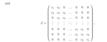
withc1=1+D4∆t/(∆x)2+∆t(µ+δ+γ),c2=−D4∆t/(∆x)2andc3=1+2D4∆t/(∆x)2+∆t(µ+δ+γ).Since C is a M-matrix,one has

Thus,the solution of system(3.1)remains nonnegative.

4 Global Stability of the Discretized System(3.1)

In this section,we discuss the global stability of equilibria for system(3.1).

Theorem 4.1For any∆x>0 and∆t>0,if R0≤1,thenE0of system(3.1)is globally asymptotically stable.

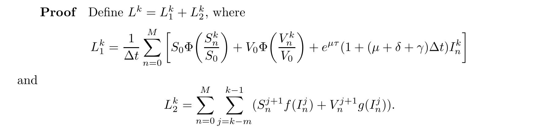
Clearly,Lk≥0 with equality holds if and only iffor allk∈N andn∈{1,2,...,M}.

ApplyingµpA=(µ+α)S0,µqA+αS0=(µ+β)V0,we can get

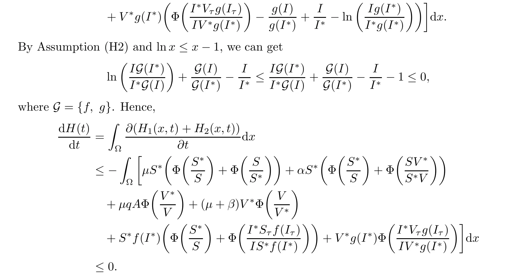
Theorem 4.2For any∆x>0 and∆t>0,if R0>1,thenE∗of system(3.1)is globally asymptotically stable.

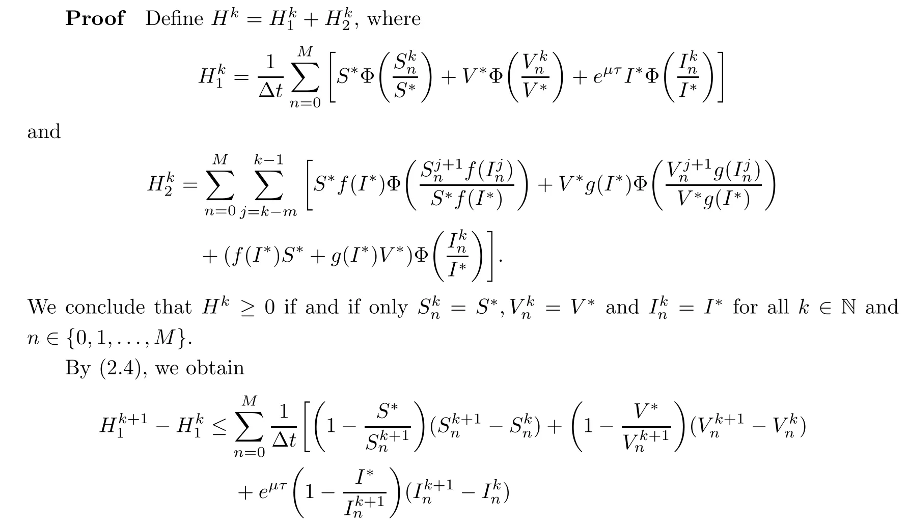
Applying Assumption(H2)and that lnx≤x−1,we can get

where G={f,g}.Therefore,

5 Numerical Simulations

By(2.3)and simple calculations,we have that R0=0.9278<1 and thatE0=(77.4336,7743.3628,0).Using Theorem 4.1,E0is globally asymptotically stable.One gets that the disease is extinct(see Figure 1).

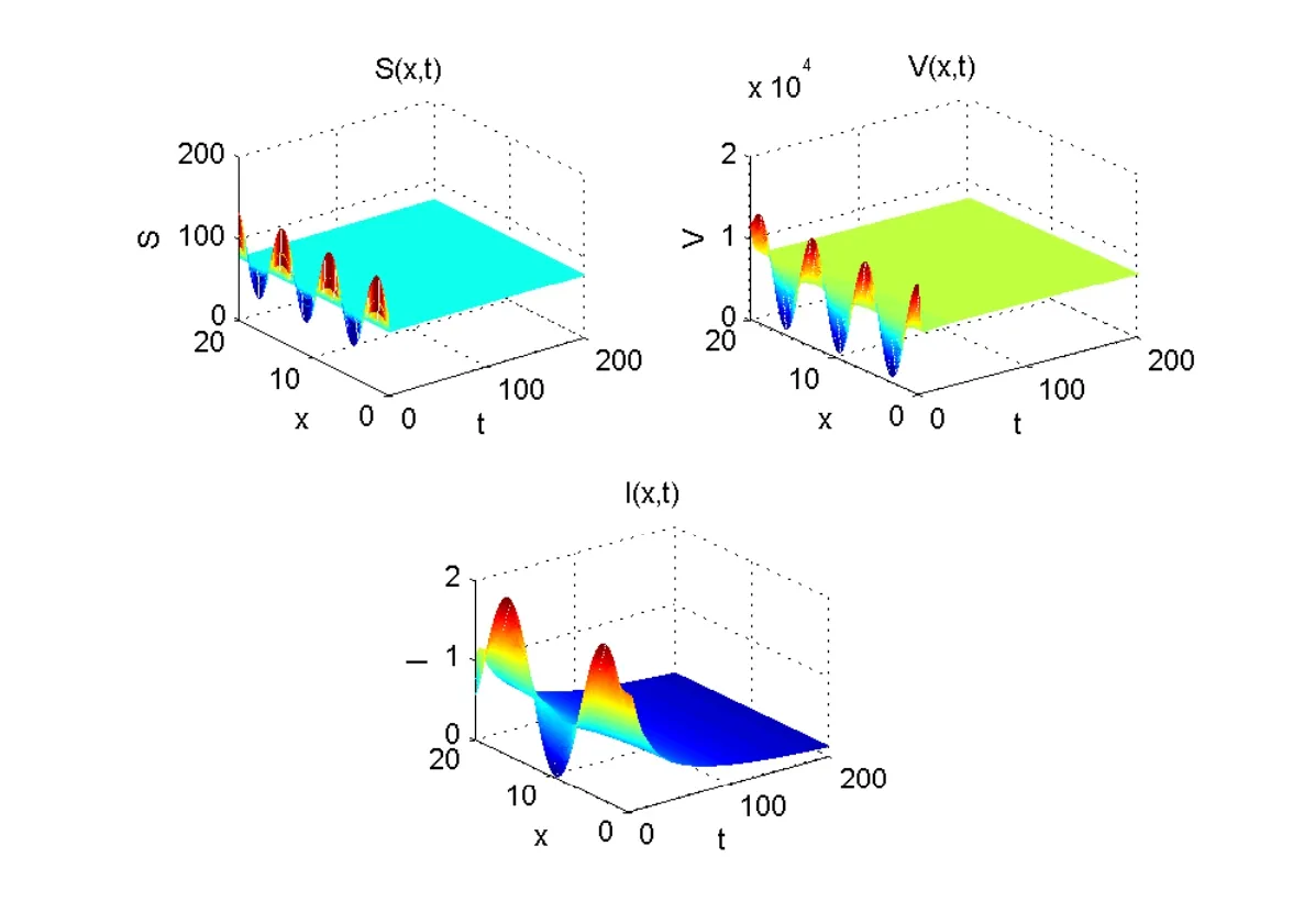
Figure 1 The disease-free equilibrium E0=(77.4336,7743.3628,0)of system(3.1)is globally asymptotically stable when R0=0.9278<1

Case 2Chooseα=0.9,τ=20 and initial condition

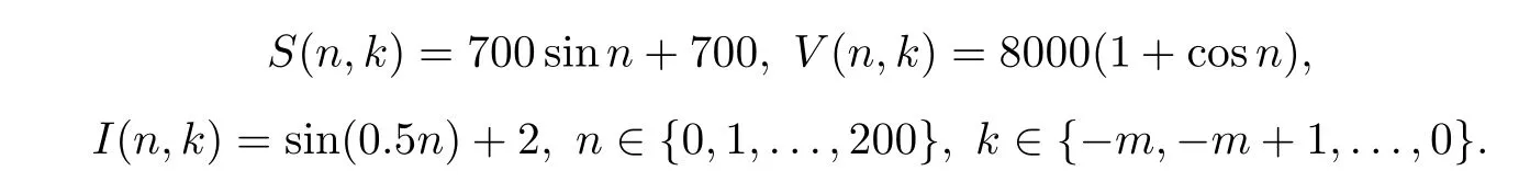
We obtain that R0=2.8999>1 and thatE∗=(744.4733,7444.0831,1.8991),respectively.Thus,E∗is globally asymptotically stable,by Theorem 4.2.Hence,the disease will eventually become endemic(see Figure 2).

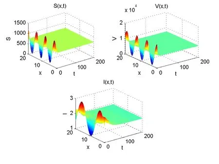
Figure 2 The disease-free equilibrium E∗=(744.4733,7444.0831,1.8991)of system(3.1)is globally asymptotically stable when R0=2.8999>1

Case 3Effect of time delay.

Chooseτ=5,10,15,20 withα=0.9 and an initial condition as in Case(2).We obtain that R0=5.2840,4.3262,3.5420,2.8999 and thatI∗=4.2821,3.3247,2.5408,1.8991,respectively.Here,we give the simulations of solutions of the infectiousIatx=10 with different values ofτ.We observe that the number of those who are infectious decreases with an increase ofτ(see Figure 3).Biologically,this delay can play an important role in eliminating the number of people who are infectious.By increasing the delay,we can decrease the number of people who are infectious.

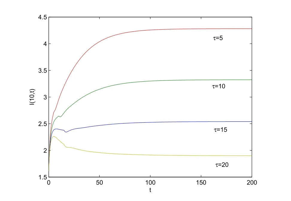
Figure 3 The solutions of the infectious I at x=10 with different τ in Case(3)

6 Conclusions

In this paper,we proposed a diffusive SVEIR epidemic model with time delay and general incidence.For this model,we first considered the global dynamics of the continuous case.Then,by using the NSFD scheme,we derived the discretization of the model.It has been shown that the global stability of the equilibria is completely determined by the basic reproduction number R0:if R0≤1,then the disease-free equilibriumE0is globally asymptotically stable;if R0>1,then the endemic equilibriumE∗is globally asymptotically stable.One sees that the NSFD scheme can preserve the global properties of solutions for an original continuous model,such as the positivity and ultimate boundedness of solutions,and global stability of the equilibria.It is our intention to use this method to study other delayed diffusive epidemic models.