
Theory of unconventional superconductivity in nickelate-based materials∗
2021-10-28 07:03MingZhang张铭YuZhang张渝HuaimingGuo郭怀明andFanYang杨帆
Chinese Physics B 2021年10期
关键词:杨帆
Ming Zhang(张铭) Yu Zhang(张渝) Huaiming Guo(郭怀明) and Fan Yang(杨帆)
1School of Physics,Beijing Institute of Technology,Beijing 100081,China
2Institute for Quantum Science and Engineering and Department of Physics,Southern University of Science and Technology,Shenzhen 518055,China
3School of Physics,Beihang University,Beijing 100191,China
Keywords: nickelate superconductor,pairing symmetries
1. Introduction
The discovery of superconductivity(SC)with highestTcup to 15 K in the Sr-doped infinite-layer nickelate NdNiO2[1,2]has attracted great research interests both experimentally[3–7]and theoretically.[4,8–26]This superconductor was thought to be a Ni-based analogy of the hight-temperature cuprates superconductors:[2]the 3d9electronic configuration of the Ni+in the NdNiO2is similar to that of the Cu2+in the cuprates; both compounds have isostructural CuO2/NiO2plane withD4symmetry. Density functional theory (DFT)based calculations[12]suggest that the electron–phonon coupling mediated pairing mechanism cannot account for theTcas high as 15 K, and the SC in this material is more likely driven by electron–electron interactions. More remarkably, recent doping study over the parent compound reveals a dome-shaped dependence of the superconductingTcover the doping concentration,[5,6]which is similar to that of the cuprates. These similarities between the Sr-doped NdNiO2and the cuprates superconductors imply that the study on the former is helpful for the clarification of the pairing mechanism of the high-temperature cuprate superconductors.[27]
There are, however, significant differences between the cuprates and the infinite-layer nickelate.[2]One difference lies in the presence of the small Fermi-pockets around the Aand possibly theΓ-points in the Brillouin zone in the parent compound NdNiO2, which are mainly contributed from the 5d electrons of the Nd.[8,11–14,19,22–26]These Nd 5d-stateoriginated Fermi pockets lead to self doping into the shouldbe Mott-insulating NiO2plane with extra holes. Note that the charge-transfer gap between the Ni 3d states and the O 2p states in the NdNiO2is much larger than that in the cuprates,[2,7,9,21,24]which indicts that the extra holes in the NiO2plane should locate on the Ni 3d orbitals instead of the O 2p ones. Therefore, the Zhang–Rice singlet[28]present in the cuprates is absent here. These conducting Nd 5d electrons and the extra holes in the NiO2plane make the NdNiO2metallic. The other obvious difference lies in that, unlike the cuprates, the parent compound NdNiO2is not antiferromagnetic (AFM) ordered.[2,29,30]One possible reason lies in that the AFM superexchange interaction in the NdNiO2is much weaker than that in the cuprates.[2,7]The other reason lies in that the Kondo coupling between the conduction Nd 5d electrons and the localized Ni 3d electrons leads to formation of the Kondo singlet at low temperature,[2,13,14,16,23,24]which suppresses the AFM order. Therefore,the main difference between the cuprates and the infinite-layer nickelate might lies in the presence of the low-lying Nd 5d degree of freedom in the parent compound. Such difference will be largely suppressed with the enhancement of the hole doping,[11,12,15,25]as the participation of the Nd 5d electrons in the low-energy physics simply takes the form of electron pockets, which will vanish or shrink upon hole doping. Therefore,as long as the pairing mechanism and pairing symmetry in the Sr-doped compound are considered,the Ni 3d electrons should take the main role.
The band structure of the NdNiO2has been studied previously.[31–33]To make the succeeding calculations considering electron–electron interactions realizable,a tight-binding(TB) model with finite-range hopping integrals is required.In the TB model introduced in Ref. [22], all the orbitals involved on the FS are considered, which leads to a seven- or six-orbital model. Such a model can provide a perfect description of the band structure of NdNiO2. Then a fluctuationexchange study on this model yields the dx2−y2pairing symmetry. Here to make the physics more simple and clear, we start from a two-orbital TB model provided in Ref.[4]. In this model, only the Nd 5d orbital and the Ni 3dx2−y2orbital are considered. As the hybridization between the two orbitals is weak,[4]we perform two comparison studies on the model: in one study we adopt the realistic band structure with weak coupling between the two orbitals, in the other one we turn off the coupling and study the imaginary comparison model. Our random-phase-approximation (RPA) based calculations yield very similar results for the two studies: both studies yield the dx2−y2pairing symmetry consistent with that obtained in other studies,[11,22,24]and the spin correlations obtained in the two studies are very similar: both studies reveal strong inplane spin fluctuations,consistent with Refs.[17,20]. In both studies, either the Cooper pairing or the spin fluctuations are mainly carried out by the Ni 3dx2−y2orbital. Our results suggest that the Sr-doped NdNiO2superconductor is essentially a single Ni-3dx2−y2-orbital system, and the only role of the Nd 5d orbital is to slightly tune the doping concentration of the charge carrier. More interestingly, our study can well reproduce the dome-shaped dependence of theTcover the Sr-doping concentration revealed in the recent experiment,[5,6]implying the relevance of our study to the real material.
The rest of this paper is organized as follows. In Section 2, we describe the adopted TB model. In Section 3, we introduce the details of the RPA approach engaged in our calculations. In Section 4,we provide the results of our numerical calculations:we study both cases of realisticVR,Ni/=0 and imaginaryVR,Ni=0 for comparison. HereVR,Ni(R=La,Nd)represents the hybridization between the Ni-3dx2−y2orbital and theR-5d orbital. It will be seen that the two cases yield very similar results, and that the Ni-3dx2−y2orbital takes the main role in determining the low-energy physics of the system.Finally,in Section 5,conclusions are reached with further discussions.
2. The model
TheRNiO2(R=La,Nd)has a body-centered cubic structure with the lattice constantsa=b/=c. In the cubic unit cell,R(Ni) is at the vertex (center) of the cube, and O is in the middle of each face. The band structures of LaNiO2and NdNiO2are very similar, in which only the 3dx2−y2orbital of Ni and the 5d orbitals of La or Nd play the main role near the Fermi energy.[4,11]Here we start from a minimal twoband tight binding model[4]to describe the low-energy physics dominated by the rare-earthRand Ni bands,which writes as
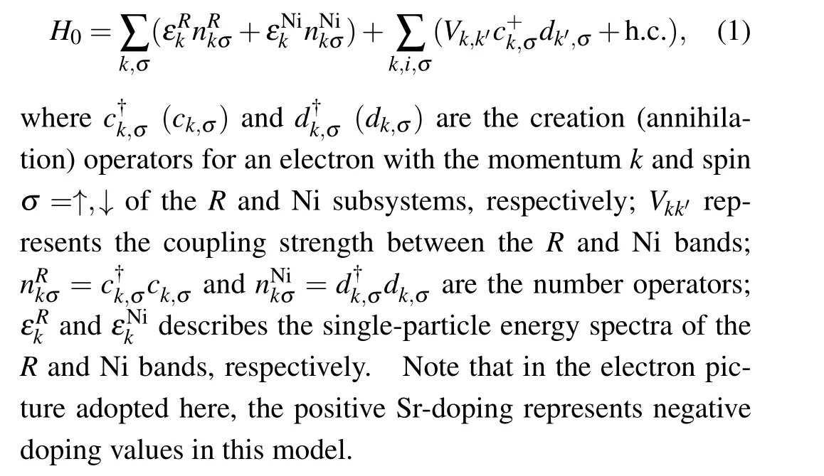
We take the relevant parameters from Ref.[4],and show the band structure of the Hamiltonian(1)in Fig.1. Note that although the provided TB parameters are for LaNiO2,the obtained band structure can also well describe the band structure of NdNiO2, as the band structures of the two materials are very similar. Here only the Ni 3dx2−y2and La 5d3z2−r2orbitals are considered for simplicity. In this system, although the Ni 3d orbital and the La 5d orbital are coupled through hybridization, such coupling is on the order of O(10−2) eV,which is negligibly small compared to the intra-layer hopping amplitudes. Therefore, each of the two resulting bands has a dominating orbital component. The Ni 3d-orbital dominated band is almost dispersionless alongΓ–Z(thez-axis in the Brillouin zone), and hence it is of two-dimensional (2D)nature. In contrast,the La 5d-orbital dominated band is quite extended and three-dimensional (3D). Specially two small Fermi surface pockets are formed at theΓand theApoints,based on this 3D band. For comparison purpose,we also calculate the band structure with the inter-orbital hybridization turning off, i.e.,Vkk′=0, in which the two bands are completely decoupled. As shown in Fig. 1(b), the resulting band structure is almost identical to that in Fig.1(a),and all features are remained.

Fig. 1. Band structure of the Hamiltonian in Eq. (1): (a) the realistic case with weak inter-orbital coupling; (b) the comparison case with the interorbital coupling turning off. In(a)((b)),the red one is mainly(completely)composed of R 5d, and the blue one is mainly (completely) composed of Ni 3dx2−y2. (c)The high symmetry points in the tetragonal Brillouin zone.The two dashed lines are the chemical potentials corresponding to doping 0 and doping −0.2,respectively.
The density of states (DOS) of the system is shown in Fig. 2(a), with the contributions from the two orbital components marked separately. From Fig.2(a),it is clear that for the undoped parent compound, the most part of the DOS is contributed by the Ni 3dx2−y2orbital,with theR5d orbital slightly contributing to the DOS.Further more,when the compound is hole-doped by substituting someR3+ions with Sr2+atoms,the part contributed by theR5d orbital continues decreasing and vanishes promptly. On the contrary, the part of the DOS contributed by the Ni 3dx2−y2orbital increases promptly upon the hole-doping, and experiences a 3D VHS (introduced below)at the dopingδc=−0.1. After that the DOS decreases,leading to a dome-shaped curve for the DOS contributed by the Ni 3dx2−y2orbital,as shown in Fig.2(a). When the parent compound is electron-doped, the situation becomes very different: the part of the DOS contributed by the Ni 3dx2−y2orbital decreases promptly,while that contributed by theR5d orbital orbital increases. The DOS for the comparison model with the inter-orbital coupling turning off is shown in Fig.2(b),which can not be obviously distinguished from Fig.2(a).
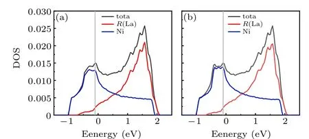
Fig. 2. DOS of the Hamiltonian in Eq. (1): (a) the realistic case; (b) the comparison case. The contribution to the DOS from each orbital component is also marked,with the red one marking the La 5d component and the blue one marking the Ni 3dx2−y2 one.The grey vertical line marks the VH doping level,which is equal to −0.1 for(a)and −0.11 for(b).
The 3D Fermi surface (FS) of the model is shown in Fig. 3(a) for the undoped parent compound and Fig. 3(b) for the hole-doped case with doping levelδ=−0.2 where theTcof the SC is the highest. For the zero doping, the FS includes a 2D columnar sheet centering around theM–Aline whose main orbital component is the Ni 3d orbital, and two 3D spherical Fermi pockets centering around theΓand theApoints respectively whose main orbital component is theR5d orbital. While the Ni-3d-orbital derived 2D FS column is hole pocket,the twoR-5d-orbital derived pockets are electron pockets. Forδ=−0.2, the two electron pockets contributed mainly from theR-5d-orbital greatly shrink,with theΓpocket nearly invisible. In the meantime,the columnar“hole pocket”formed mainly by the Ni-3d-orbital expands obviously with hole-doping until its top part near thekz=πplane experiences a Lifshitz transition and changes its topology,as is more clear in the 2D FS shown below.
The 3D FSs for the comparison band structure with the inter-orbital coupling between the Ni 3d andR-5d-orbitals turning off are shown in Fig. 3(c) for the undoped case and Fig. 3(d) forδ=−0.2, which cannot be obviously distinguished from the uncoupled case shown in Figs.3(a)and 3(b).
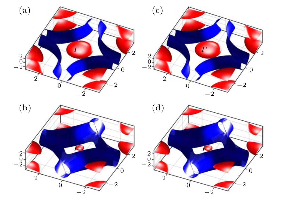
Fig. 3. The 3D FSs for the realistic band structure at the doping levels (a)δ =0 and(b)δ =−0.2;and those for the comparison band structure at the doping levels(c)δ =0 and(d)δ =−0.2.
The 2D FS for the zero doping is shown in Fig. 4(a) forkz= 0 and 4(b) forkz=π, while that for the doping levelδ=−0.2 is shown in Figs. 4(c) and 4(d). Figures 4(a) and 4(b) reveal the two separateR5d-orbital derived 3D electron pockets centering at theΓandApoints,and the Ni 3d-orbital derived 2D columnar FS surrounding theM–Aline which can be regarded as a hole pocket. Clearly, the cut of this Ni 3d pocket on thekz=πplane hosts a larger area than that on thekz=0 plane. When the doping is shifted toδ=−0.2,the twoR5d-orbital derived 3D electron pockets shrink a lot,with theΓ-pocket almost invisible. In the meantime,the Ni 3d pocket expands a lot,as shown by Figs.4(c)and 4(d).Such expansion is more clear on thekz=πplane, where the different sheets of the hole pocket which used to surround theApoint atδ=0 now touch with each other and the FS on this plane has now changed to an electron pocket surrounding theZpoint. Such a FS-topology change on thekz=πplane suggests that the system has experienced a Lifshitz transition,which takes place at the doping levelδc=−0.1. Such a Lifshitz transition makes a van Hove singularity(VHS),with the VH momenta locating at theR-points. Such a VHS on the FS has enhanced the DOS,leading to a broad peak in the DOS curve shown in Fig.2. The 2D FS and its evolution with doping for the comparison band structure with the inter-orbital coupling turning off(un-shown)cannot be obviously distinguished from Fig.4.
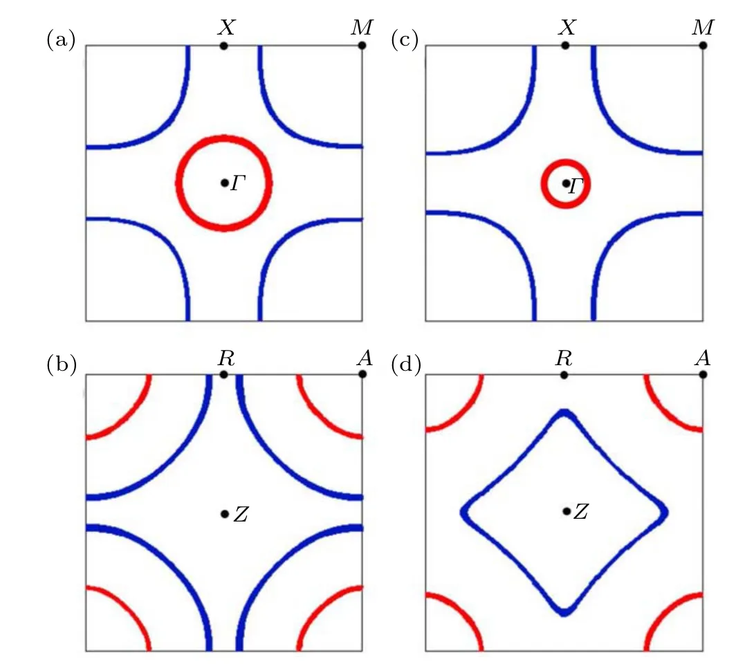
Fig.4. The 2D FSs for the doping levels δ =0 on the kz=0 plane(a)and kz =π plane (b), and those for the doping levels δ =−0.2 on the kz =0 plane(c)and kz=π plane(d). Only the results for the realistic band structure are shown.
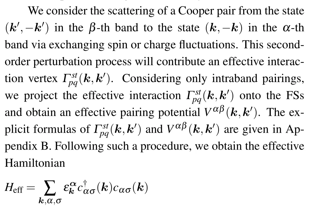
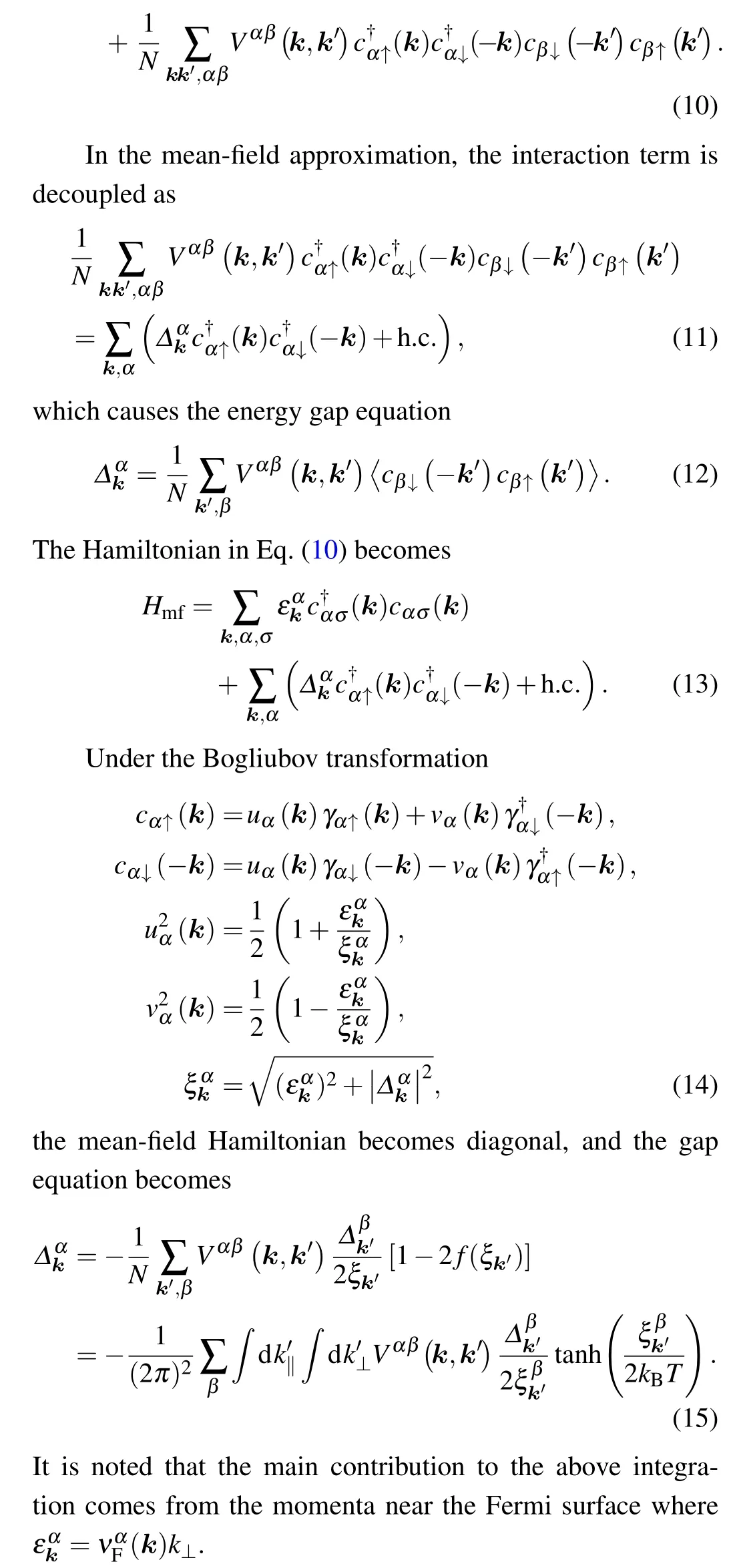
3. The RPA formulation


Generally, repulsive Hubbard interactions suppress the charge susceptibility,but enhance the spin susceptibility.[34–46]There is a critical interaction strengthUc,where the spin susceptibility diverges, indicating that the long-range magnetic order forms,and the RPA treatment is no longer valid.[47–50,52]When the interaction strength is belowUc, short-ranged spin and charge fluctuations exist in the system. Electrons may form Cooper pairs by exchanging these fluctuations,resulting in exotic superconducting states in the system.

According to theD4hpoint group[53]of LaNiO2, the possible superconducting pairing symmetries include A1g(s)-,Eu(p)-,B1g(dx2−y2)-,B2g(dxy)-,A2g(dx2−y2×dxy)-,A2u(pz)-,Eg(px×pz/py×pz)-, B2u(dx2−y2×pz)-, B1u(dxy×pz)- and A1u(dx2−y2×dxy×pz)-wave ones. The eigenvector(s)Δα(k)for each eigenvalueλobtained from gap equation(17)as the basis function(s)forms(form)an irreducible representation of theD4hpoint group. While the Eu(p), Eg(px×pz/py×pz)symmetries each form a 2D representation with degenerate pairing eigenvalues,other symmetries each forms a 1D representation of the point group with nondegenerate pairing eigenvalues. The character table for each representation of theD4hpoint group is shown in Table 1.
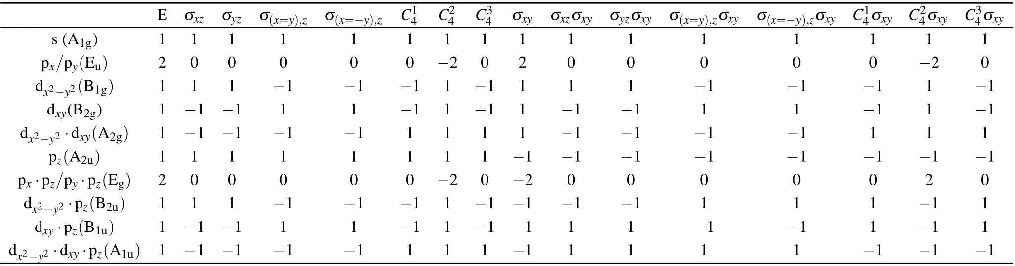
Table 1. The D4h character table.
4. Numerical result
In this section, we present our numerical results for the spin correlations and pairing symmetries in this system. We compare the results obtained for two cases: one case is for the realistic band structure with weak inter-orbital coupling between the Ni 3d and La 5d orbitals, and the other one is for the imaginary comparison band structure with no coupling between the Ni 3d and La 5d orbitals. Our results suggest that the spin correlations obtained for the two cases are similar,and the pairing symmetries obtained are both dx2−y2which is robust against doping. Our results suggest that the pairing mechanism and pairing symmetry of this system are mainly determined by the 3d orbital of Ni,and the main role of La is only to adjust the effective doping concentration. In the following,we provide our results for both cases simultaneously.For the doping levels, we provide two cases for comparison:one is zero doping, and the other is−0.2 which represents a typical doping level with obviousTcfor the SC. The 3D and 2D FSs for the two doping levels are shown in Figs.3 and 4,respectively.
In Fig. 5, we show thekdependence of the susceptibilityχ(k) in the Brillouin zone. Hereχrepresents the largest eigenvalue of the susceptibility matrix (χ). The elementχlm(k)of this matrix is defined as
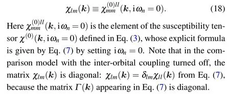
Theχ(k)for two typical doping levels,i.e.,0 and−0.2,are shown in Fig. 5. For the zero doping, such momentum dependence is shown along the high-symmetry lines in the Brillouin zone in (a), on thekz=0 plane in (b), and on thekz=πplane in (c). Clearly, there are two peaks for the distribution ofχ(q), with one near theM=(π,π,0) point, and the other near theA=(π,π,π) point. The in-plane component of both momenta is(π,π),reflecting the strong in-plane antiferromagnetic(AFM)spin correlations. The two peaks are nearly degenerate, reflecting the competition between interlayer AFM and FM correlations. When the doping concentration is changed to−0.2,such momentum dependence is shown in Figs.5(d)–5(f). In this doping level,there are still two susceptibility peaks near theMandApoints. However, theApeak is slightly higher than theM-peak, reflecting that while the in-plane spin correlation is still AFM, the inter-layer one is also AFM.Similarkdependence ofχ(k)for the comparison band structure with the inter-orbital coupling turning off is shown in Fig.6. A comparison between Figs.5 and 6 reveals that the two figures are nearly the same,suggesting that the influence of the inter-orbital coupling between the Ni 3d orbital and theR5d orbital on the spin correlations in this system can be ignored.
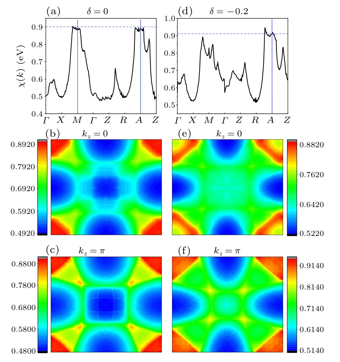
Fig.5. The k-space distribution of the largest eigenvalue χ(k)of the susceptibility matrix for the realistic band structure.Of which,(a),(b),(c)represent the doping 0 and(d),(e),(f)represent the doping −0.2. (a)and(d)are along the high-symmetry lines in the Brillouin zone, (b)and(e)are on the kz =0 plane,and(c)and(f)are on the kz=π plane.

Fig.6. The k-space distribution of the largest eigenvalue χ(k)of the susceptibility matrix for the comparison band structure with the inter-orbital coupling turned off. The meaning of each figure is similar to that in Fig.5.
From the eigenvectorξ(km)corresponding to the largest eigenvalueχ(km) of the susceptibility matrix atkm, the spin fluctuation in the system takes the pattern ofsiµ=ξµ(km)eikm·ri. The spin-fluctuation pattern thus obtained for the doping levelδ=−0.2 is shown from top view in Fig.7(a)and from side view in Fig. 7(b). As thekmfor this doping level is atA,the obtained spin-fluctuation pattern is the Neelordered AFM pattern both intra-layer and inter-layer. What’s more, the distribution ofsiµbetween the two orbitalsµ=1 andµ=2 is determined byξµ(km).From our calculation,it is obtained asξ1(km)/ξ2(km)=10−4, which is very small. As a result,the spin fluctuation is mainly carried by the Ni 3d orbital,as shown in Figs.7(a)and 7(b). Similar spin-fluctuation patterns thus obtained for the comparison case with the coupling between the Ni 3d and theR5d orbitals turning off are shown in Figs.7(c)and 7(d)for the top and side views,respectively. In Figs. 7(c) and 7(d), the spin pattern is completely distributed on the Ni 3d orbital asξ1(km)=0,ξ2(km)=1,suggesting that if we omitted the inter-orbital coupling the spin fluctuation should be completely carried by the Ni 3d orbital. Comparing the case with realistic weak inter-orbital coupling between the Ni 3d andR5d orbitals and the one without such inter-orbital coupling, it is known that the spin fluctuation in this system is mainly carried by the Ni 3d orbital and theR5d orbital only participates into the spin fluctuation through the tiny hybridization with Ni 3d orbital.

Fig. 7. The spin-fluctuation pattern, in which blue color represents Ni and the red one represents La. (a),(b)are top view and side view for the realistic band structure with weak inter-orbital coupling and(c),(d)are top view and side view for the comparison band structure with the inter-orbital coupling turned off. The doping for both cases is −0.2. The relative ratio between the lengths of the arrows representing the spins of the two orbitals has been exaggerated.
When the interaction strength is below the critical one,the above illustrated spin fluctuation is short-ranged. Through exchanging these short-ranged spin fluctuations,a pair of electrons with opposite momenta can acquire effective attraction and pair, which leads to the SC. In our calculations, we takeU=0.9 eV,under which the renormalized spin and charge susceptibilities do not diverge,which suggest that this interaction strength is below the critical one. The pairing phase diagram thus obtained is shown in Fig. 8. Figure 8 suggests that the phase diagram (a) for the realistic band structure with weak inter-orbital coupling between Ni 3d andR5d and that(b)for the comparison band structure with the inter-orbital coupling turning off are very similar. Figure 8 reveals three experimentally relevant characters in the doping dependence of the pairing phase diagram.
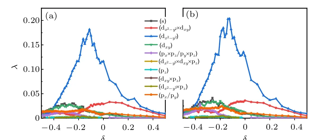
Fig. 8. Doping δ dependence of the largest pairing eigenvalue λ for each pairing symmetry for the realistic band structure (a) and the comparison band structure(b).
Firstly, the pairingTcfor the hole-doped case is much larger than that for the electron-doped case. Particularly, theTcfor the electron-doped case decreases promptly with doping, which might possibly be invisible in experiment. This character is different from that of the cuprates superconductors which host high-temperature SC for both hole-doped and electron-doped cases and is consistent with the experiment of the Sr-doped NdNiO2superconductors wherein the Sr doping introduced holes into the material. The physical reason in our study for this character lies in that,on the one hand the Ni 3d orbital-component contributes less and less to the DOS of the electron-doped case,and on the other hand it is the Ni 3d orbital-component which contributes to the SC of the material,as more clearly illustrated below. Our study thus predicts that no obvious SC would be detected for the electron-doped case of the NdNiO2.
Secondly, the pairingTcfor the hole-doped case exhibits a dome shape, which peaks in between the doping levels−0.1 and−0.2. Such a dome-shaped curve of the doping-dependentTcis qualitatively consistent with recent experiments[5,6]wherein the peak of theTcis near the doping−0.2. The physical reason of this character lies in that,the Ni 3d-orbital component of the DOS, which contributes mainly to the SC of the system,peaks near this doping range,as shown in the DOS curve in Fig. 2. This DOS peak originates from the VHS caused by the Lifshitz transition of the FS,as shown in Fig.9. Figures 9(a)and 9(b)show the 2D FS on thekz=0 andkz=πplanes for the VH dopingδc=−0.1 for the realistic band structure. This 2D FS can be compared with those forδ=0 andδ=−0.2 shown in Fig. 4.Clearly, while the 2D FSs for the three cases on thekz=0 plane have the same topology,those on thekz=πplane illustrate a FS-topology change. While the FS on thekz=πplane forδ=0 shown in Fig.4(b)comprises aR5d-orbital derived electron pocket and a Ni 3d-orbital derived hole pocket centering around theApoint, that forδ=−0.2 shown in Fig. 4(d)comprises two electron pockets,with the Ni 3d-orbital derived FS sheet now changing topology to an electron pocket centering around theZpoint. Clearly, the Ni 3d-orbital derived FS sheet has experienced a Lifshitz transition fromδ=0 toδ=−0.2. Figure 9(b) just illustrates the Lifshitz transition point atδc=−0.1,on which the separate FS sheets appearing in Fig. 4(b) now touch with each other at theR-points, making these points as the VH momenta. This 3D VHS will not lead to a divergence of the DOS, but it causes a broad peak in the DOS in Fig.2(a),which just leads to the broadTc-peak in Fig. 8(a). The situation for the comparison band structure(δc=−0.11)shown in Figs.9(c)and 9(d)is similar,which is related to the broadTc-peak in Fig.8(b).
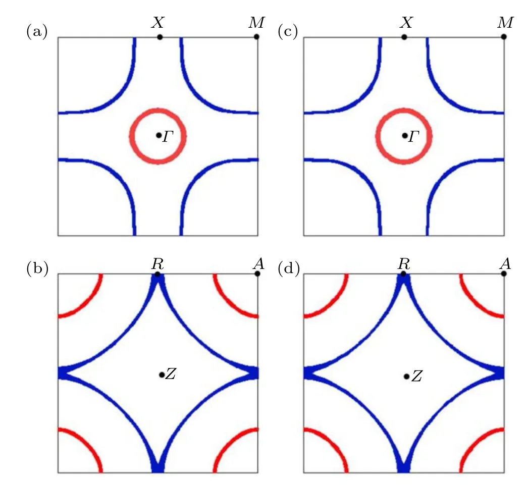
Fig.9.The 2D FS of the VH doping(δc=−0.1)for the realistic band structure on the kz=0 plane(a)and kz=π plane(b),and that(δc=−0.11)for the comparison band structure on the kz=0 plane(c)and kz=π plane(d).
Thirdly, while all the ten possible pairing symmetries listed in Table 1 are possible, the dx2−y2-wave pairing dominates over other pairing symmetries in the whole doping range where obvious SC can be detected. This robust dx2−y2-wave pairing obtained for our simple model is consistent with those obtained for more complicated models.[11,22]The distribution of the gap function for the obtained dx2−y2-wave pairing on the FS is shown in Fig. 10(a) on thekz=0 plane and Fig. 10(b)on thekz=πplane for the doping levelδ=−0.2. Obviously, this gap function is symmetric about thexandyaxes and is antisymmetric about thex=±yaxes. Four symmetryprotected line nodes are presented in the 3D Brillouin zone whose projections on thexyplane locate on thex=±yaxes.It is also obvious that the pairing gap is mainly distributed on the Ni 3d-orbital derived FS sheets,with the component on theR5d-orbital derived FS sheets almost vanished,suggesting the dominating role of the Ni 3d orbital in determining the SC in this system. The situation for the comparison band structure is similar,as shown in Figs.10(c)and 10(d).
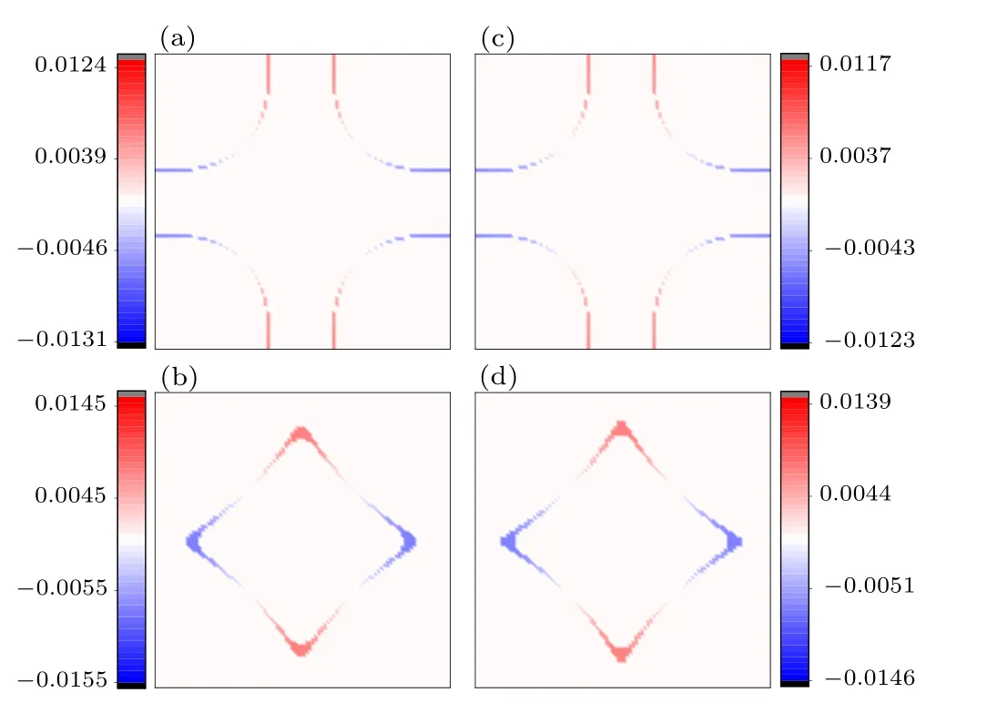
Fig. 10. Distributions of the gap functions on the FS for the doping level−0.2 for the realistic band structure(a),(b)and the comparison band structure with the inter-orbital coupling turned off(c),(d). While(a)and(c)are the distribution on the kz=0 plane,(b)and(d)represent that on the kz=π plane.
5. Discussion and conclusion
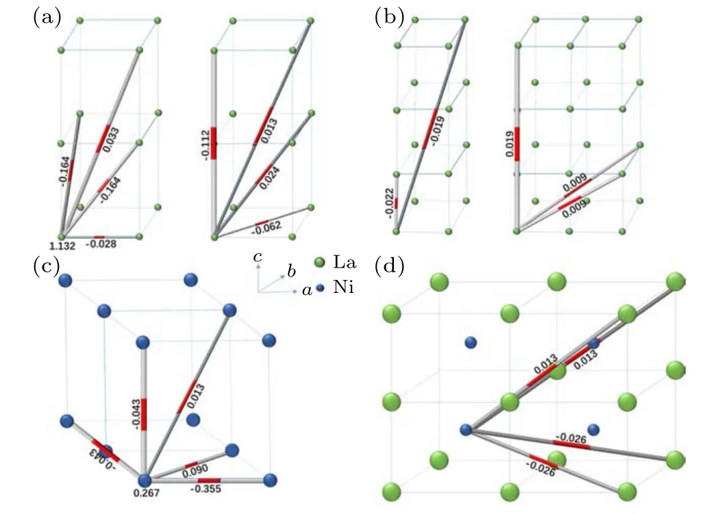
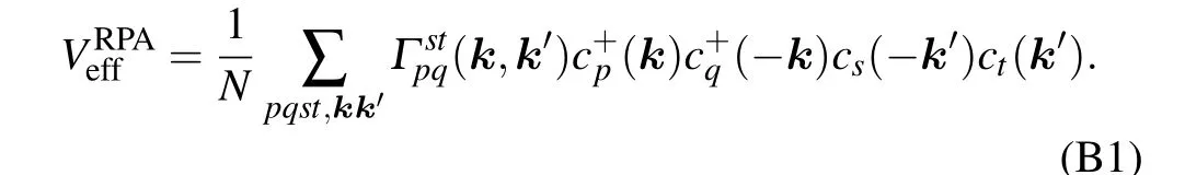
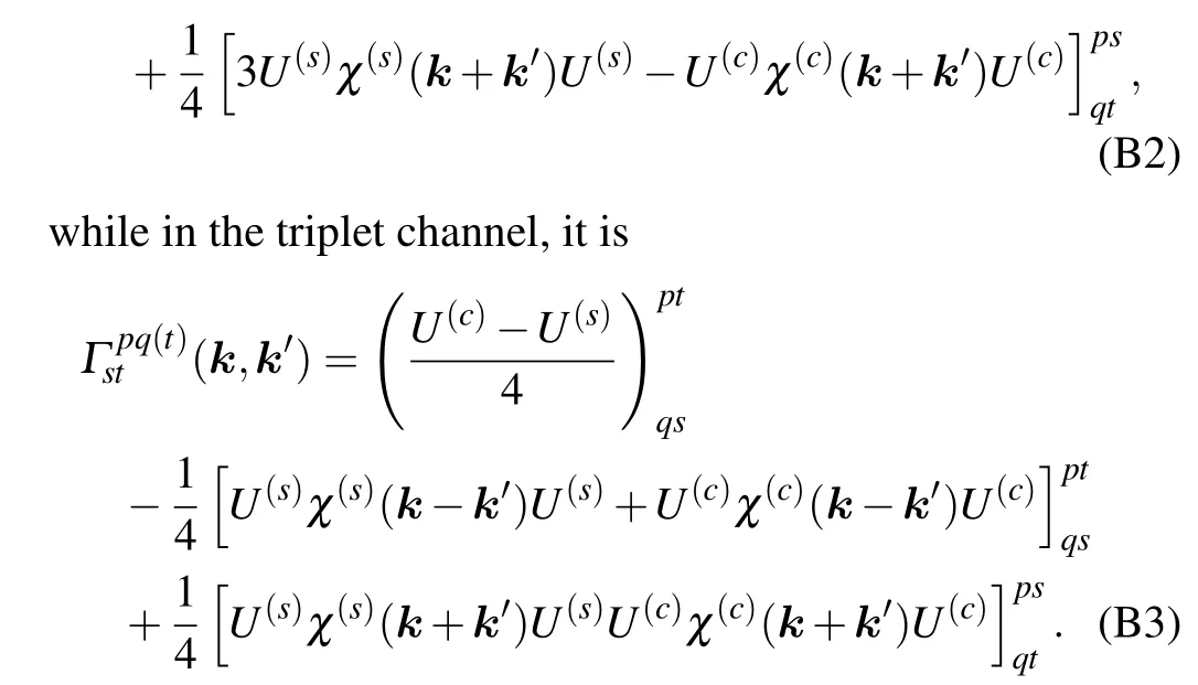
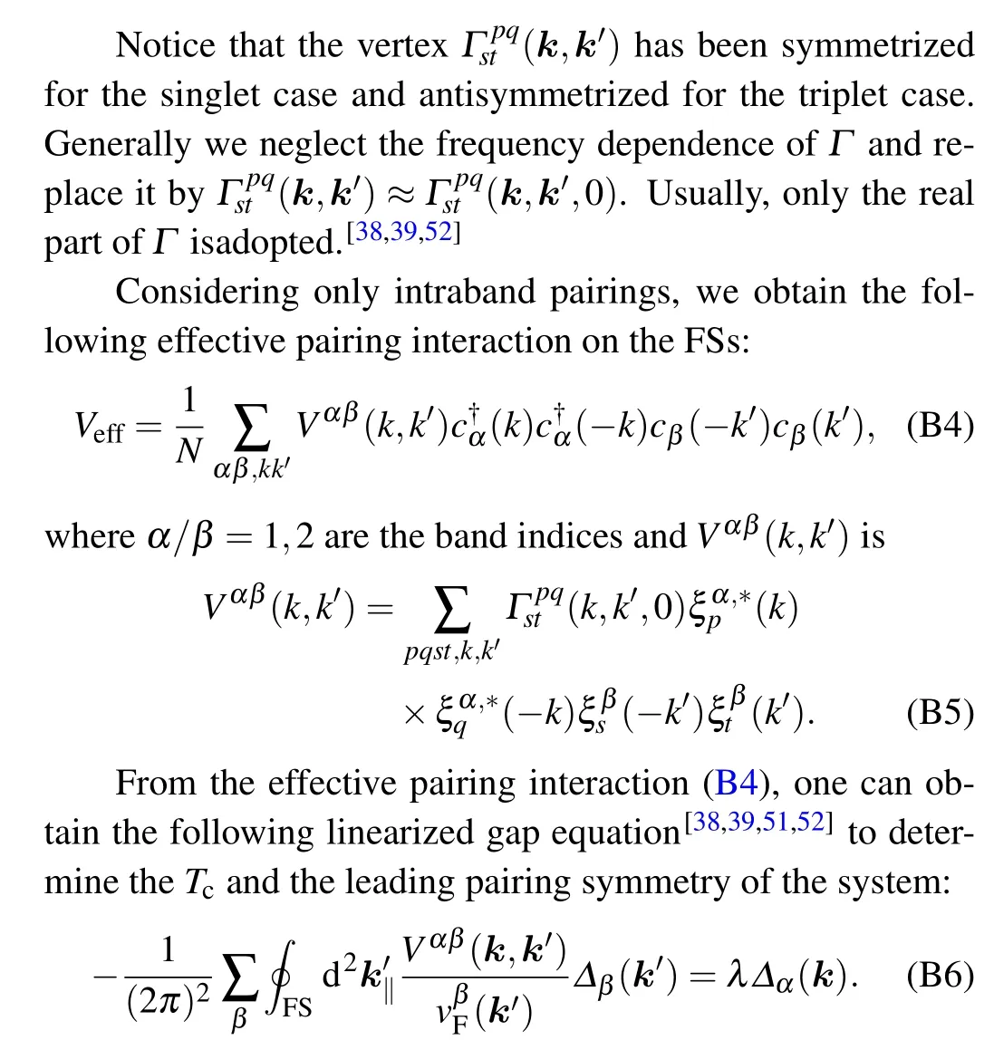
Due to the strong on-site Coulomb interaction between the Ni 3d electrons, the nickelate superconductors might belong to strongly-correlated system, or at least intermediatelycorrelated one. Here, to avoid the difficulty in the systematic treatment of strongly- or intermediately-correlated electronic systems,we start from the weak-coupling RPA approach,with the adopted Hubbard-U(0.9 eV)several times weaker than the realistic value. Two reasons lie behind this choice ofU:[34–43]on the one hand, the RPA as a perturbational approach does not apply to the case with strongU; on the other hand, the conditionU Note that the weak-coupling RPA approach adopted here might have missed the Kondo physics at the small doping levels, where the Kondo coupling between the Ni-3d and theR-5d orbitals might lead to the d+is-wave pairing.[13]However,when the hole-doping levels are large, due to the electronpocket character of theR-5d dominant FSs, the DOS contributed by theR-5d orbital component is largely reduced,and correspondingly the Kondo physics should be suppressed.Therefore, the conclusion arrived at in our study should only be tenable for large hole-doping concentrations. In conclusion, we have performed a RPA based calculation for the Sr-doped RNiO2superconductor,adopting a realistic two-band band structure. Through comparison between the results obtained for the realistic band structure and those obtained for the imaginary band structure with the inter-orbital coupling between the Ni 3d andR5d orbitals turned off,it is revealed that the Ni 3d orbital dominates over theR5d orbital in carrying out the AFM spin fluctuation and the superconducting pairing. Our results suggest that this system is essentially a one-orbital(i.e.,Ni 3d)system,with the only role of theR5d orbital to slightly tuning the doping concentration in the hole-doped superconducting regime relevant to experiments.Therefore,this material can be well captured by a single-band Hubbard model on the square lattice. Further more,our results reveal three experimentally relevant doping-dependent behaviors of the pairing state. Firstly,the superconducting pairing is strongly particle–hole asymmetric,with obviousTconly detectable on the hole-doped side.Secondly, a dome-shaped doping dependence of the SCTcis obtained, which peaks within the regime of (−0.2,−0.1),qualitatively consistent with recent experiments. These two characters are determined by the doping dependence of the DOS contributed by the Ni 3d orbital, which is particle–hole asymmetric and peaks near the doping regime of(−0.2,−0.1),caused by the 3D VHS.Thirdly, the robust dx2−y2-wave pairing symmetry dominates over other pairing symmetries in the large doping regime,consistent with the results obtained from other more complicated models. Acknowledgement We are grateful to the stimulating discussions with Congjun Wu,Chen Lu,Lun-Hui Hu and Zhan Wang. Fig.A1. The hoping between particles in real space,and the unit of related parameters is eV. Appendix B: The effective interaction The Feynman’s diagram of RPA is shown in Fig. B1.Note that when the interaction strengthUis higher thanUc,the denominator matrixI −χ(0)(k,iwn)Usin Eq.(8)will have zero eigenvalues for someqand the renormalized spin susceptibility diverges there, which invalidates the RPA treatment.WhenU Fig.B1.Feynman’s diagram for the renormalized susceptibilities in the RPA level. Fig. B2. Three processes which contribute the renormalized effective vertex considered in the RPA, with (a) the bare interaction vertex and (b), (c)the two second order perturbation processes during which spin or charge fluctuations are exchanged between a Cooper pair. This equation can be looked upon as an eigenvalue problem, where the normalized eigenvectorδα(k) represents the relative gap function on theα-th FS patches nearTc, and the eigenvalueλdeterminesTcviaTc=cutoff energy×e−1/λ,where the cutoff energy is of order bandwidth. The leading pairing symmetry is determined by the largest eigenvalueλof Eq.(B6).


 猜你喜欢
Chinese Physics B(2022年8期)2022-08-31Chinese Physics B(2022年4期)2022-04-12影剧新作(2020年2期)2020-09-23男生女生(银版)(2016年4期)2016-08-04延河(下半月)(2015年3期)2015-10-06快乐作文·低年级(2015年6期)2015-07-22南都周刊(2015年8期)2015-05-07延河·绿色文学(2015年3期)2015-03-25
猜你喜欢
Chinese Physics B(2022年8期)2022-08-31Chinese Physics B(2022年4期)2022-04-12影剧新作(2020年2期)2020-09-23男生女生(银版)(2016年4期)2016-08-04延河(下半月)(2015年3期)2015-10-06快乐作文·低年级(2015年6期)2015-07-22南都周刊(2015年8期)2015-05-07延河·绿色文学(2015年3期)2015-03-25
