
Realizing Majorana fermion modes in the Kitaev model*
2021-11-23 07:31LuYang杨露JiaXingZhang张佳星ShuangLiang梁爽WeiChen陈薇andQiangHuaWang王强华
Chinese Physics B 2021年11期
关键词:陈薇
Lu Yang(杨露) Jia-Xing Zhang(张佳星) Shuang Liang(梁爽)Wei Chen(陈薇) and Qiang-Hua Wang(王强华)
1National Laboratory of Solid State Microstructures and School of Physics,Nanjing University,Nanjing 210093,China
2Collaborative Innovation Center of Advanced Microstructures,Nanjing University,Nanjing 210093,China
3Institute of Physics,Chinese Academy of Sciences,Beijing 100190,China
Keywords: Kitaev model,Majorana fermion modes,topological quantum computing
1. Introduction
The search for Majorana fermion (MF) modes in condensed matter systems has intrigued great interest in recent years.[1-14]One important reason is because a pair of widely separated MF bound states is immune to local perturbations and may be used for fault-tolerant quantum memory.[6]Moreover, the non-Abelian statistics that the MF states obey due to the degeneracy of such states may suggest them as components of a topological qubit and be used in quantum information processing.[6,15]
Many approaches have been proposed to realize MFs in condensed matter systems, such as fractional quantum Hall states,[7]superfluids in3He-B phase,[8]semiconductors with strong spin-orbit interaction in both 2D and 1D,[6,9]coupled quantum dots,[10,11]array of magnetic atoms on the surface of superconductors,[12]and intrinsic topological superconductors.[1,13,14]All these approaches involve superconductors in the system.
In this work, however, we discuss the realization of Majorana modes in a spin system,the Kitaev model.[16]One possible realization of MF in the Kitaev model is on the edge of a chiral Kitaev spin liquid by applying a conical magnetic field on the gapless Kitaev model.[16,18]However, the edge Majorana zero mode is embedded in other edge modes with dispersion,which makes it easy to decay to other edge modes. Another proposal to achieve Majorana zero modes in the Kitaev model is by introduction of vacancy in the Kitaev model.[19,20]In Refs. [19,20], it was shown that a single vacancy in the gapless Kitaev model results in a zero mode in the ground state. However, this Majorana zero mode is embedded in a continuum of spectrum and decays algebraically in space. For the reason, it interacts strongly with other vacancy induced zero modes and disappears even if the other zero modes are far away.[20]These Majorana zero modes are then not robust enough for quantum computing.
In this work, we propose a realization of MF modes in the Kitaev model based on the result that the Kitaev model in a weak conical magnetic field turns into an effective p+ip superconductor of spinons.[16]And it is known that vortex in a p-wave superconductor may bind a Majorana zero mode that is robust against local perturbation.[1,20,22]However,these vortex excitations are usually energy-costing.[22]In this work,we discuss the possibility to create a robust and easily manipulated Majorana zero mode in the ground state of the Kitaev model as an analog of the vortex bound Majorana zero mode in the p-wave superconductor. We consider two types of defects which may result in vortex binding (orπ-flux-binding)in the ground state of the Kitaev model. One type of defect is the vacancy in the Kitaev model with a uniform[111]magnetic field.We show that under a weak uniform[111]magnetic field,a vacancy in the Kitaev model binds a flux in the ground state which results in a Majorana zero mode that decays exponentially in space. The second type of defect we study is a locally polarized spin achieved by a local magnetic field in the Kitaev model with a weak uniform[111]magnetic field.We show that upon the full polarization of the local spin, a flux is bound to the local spin plaquette in the ground state,which also results in a robust Majorana zero mode whose wavefunction decays exponentially in space. The distribution and asymptotic behaviors of the Majorana zero modes in the above two cases are also studied in this work. In both cases, the Majorana zero modes are immune to local potential perturbations and other Majorana zero modes far away, and then may be used for braiding in topological quantum computing.
This paper is organized as follows. In Section 2,we have a brief introduction of the model. In Section 3, we study the vacancy induced Majorana zero mode in the Kitaev model with a weak uniform [111] magnetic field, including the distribution and asymptotic behavior of the Majorana zero mode in both the continuum limit and lattice model, as well as the regime in which the flux binding to the vacancy takes place in the ground state. Section 4 studies the Majorana zero mode induced by the polarization of a local spin. We show the magnetization process of the local spin by mean field theory and the flux binding in the ground state upon polarization.The distribution of the Majorana zero mode after polarization is also studied in this section. At last,we compare the Majorana zero mode bound to the vacancy with the edge Majorana modes in the system and summarize the main results in this work.
2. Model and a brief review
The Kitaev model describes bond-dependent interaction of half spins on a honeycomb lattice with Hamiltonian[16]
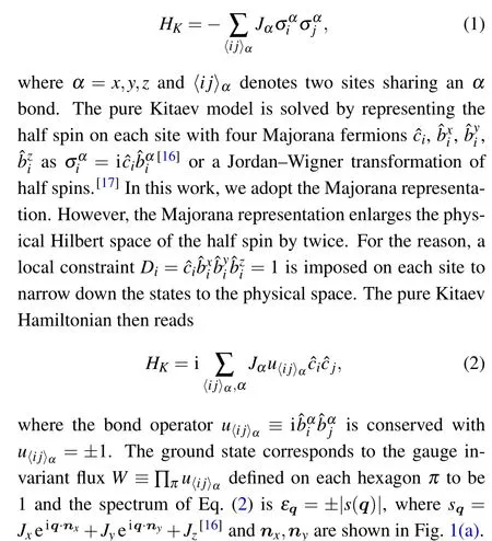
To realize Majorana zero modes in the bulk of the Kitaev lattice in this work,we first apply a[111]magnetic field to the Kitaev model, as shown in Fig. 1(a), which turns the Kitaev model to an effective px+ipysuperconductor of spinons.[16]The Hamiltonian then becomes

The uniform[111]magnetic field breaks the conservation of the flux operatorWof each hexagon plaquette. However,at weak[111]magnetic field,the most important contribution of the magnetic field comes from the third order perturbation theory[16]

where the configuration of the three neighboring sitesi,j,kis shown in Fig. 1(b) andt~h3/J2. In this work we focus on this small uniform magnetic field regime so the perturbation theory is valid and we only keep the term in Eq. (4) for the uniform magnetic field. In the Majorana representation, the Kitaev Hamiltonian including the perturbative[111]magnetic field is then[16]

where〈〈ij〉〉represents the next nearest neighborsiandjandα,β,γ=x,y,zrepresents the three bonds connected to sitek.
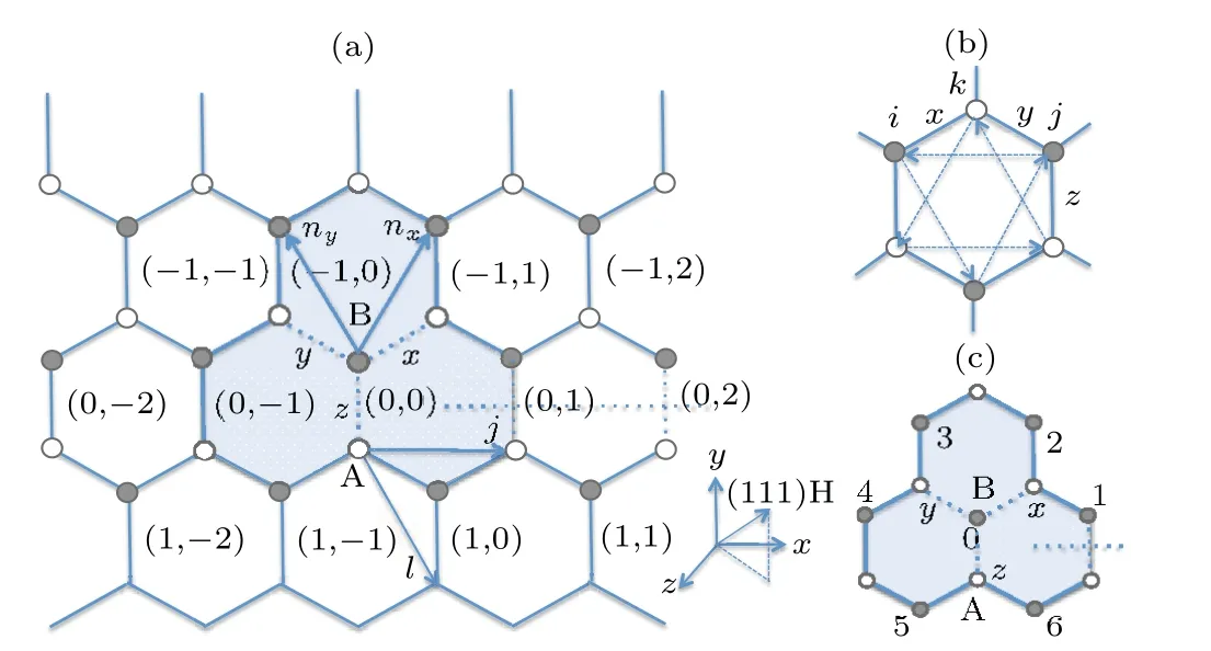
Fig. 1. (a) The honeycomb lattice and the x, y, z bonds in the Kitaev model with a vacancy site in the B sublattice at (0,0). Each unit cell contains a z bond. The flipping of bond operator u〈i j〉z on the z bonds crossing the half-infinite dashed line produces a flux/vortex in the shaded area. (b)The site index of the third order perturbation Hamiltonian in Eq.(4). The arrows indicate the hopping directions between the next nearest neighbors in the ground state. (c)Relabeling of site index with a local magnetic field applied on a B site labeled 0 in Section 4.
With only the contribution from the third order perturbation of the [111] magnetic field, the flux operatorWfor each honeycomb plaquette is still conserved. In the ground state sector,u〈ij〉α=1 and the direction of the next nearest neighbor hopping is shown in Fig.1(b). The ground state Hamiltonian is then

near the two Dirac point±qD. This Hamiltonian matrix is the same as that of a weak pairing px+ipysuperconductor,[1]though the basis here is not the Nambu spinor for superconductor but a pseudo-spinor composed of the two sublattice fields.
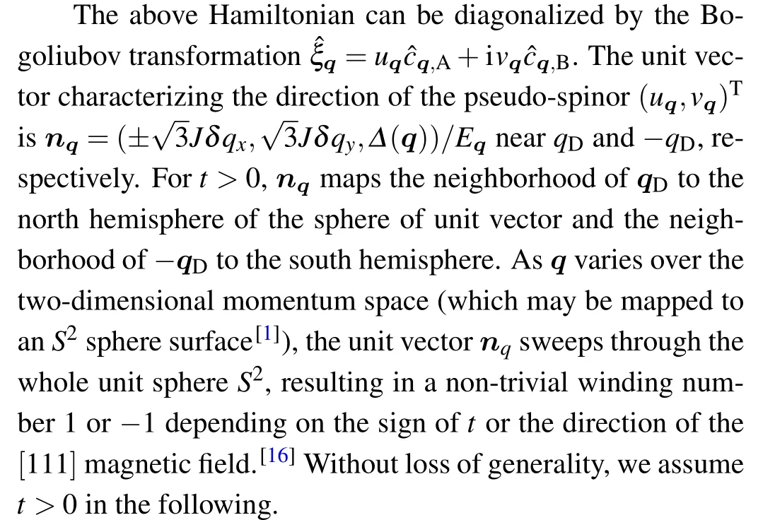
Since the Kitaev model is gapped at finitet, the Chern number of the spinon bands is well defined and may be easily computed from the eigenvectors of Eq. (8), which isν=sign∆=±1,[16]the same as a weak-pairing p-wave superconductor.
The Majorana modes in the px+ipysuperconductors have been studied extensively in previous works.[1,22,23]There are mainly two mechanisms to realize Majorana fermion modes in such systems.[1]One is on the edge of the superconductor, where the Majorana fermion modes may have both zero energy and finite energy. The other is by creating vortex in such system, since a vortex may bind a Majorana zero mode in a gapped topologically non-trivial system with odd Chern number.[16]
In the following sections,we discuss the realization of the Majorana fermion modes in the Kitaev spin liquid as an analog of the px+ipysuperconductors. We focus on the realization of the Majorana zero modes by creating vortex in the above discussed Kitaev model in the [111] magnetic field. However,the vortex is usually energy costing in such system.[22,26]Our main goal in this work is then to discuss the possibility to create vortex and Majorana modes in the ground state of this system which are suitable for braiding in topological quantum computing. For the edge mode,we only point out that for the lattice Kitaev model in the weak[111]magnetic field,only the edge mode with zero energy corresponds to a Majorana mode
whereas the chiral Majorana edge modes with finite energy only exist in the continuum limit of the Kitaev model.
3. Vacancy induced Majorana zero modes
In this section we investigate the possibility to create Majorana Fermion modes in the Kitaev model in the ground state by introducing vacancies in the Kitaev model. It has been shown in Refs.[19,20]that a vacancy in the pure Kitaev model may combine a flux in the ground state. However, a gapped pure Kitaev model has Chern number zero and there is no robust Majorana zero mode bound to the flux. For the gapless Kitaev model with a vacancy, a zero-energy resonance state was discovered.[19,20]However, this state is embedded in the bulk gapless spectrum and is easy to decay to the bulk modes.What’s more, this mode decays as a power law in space and two such modes interact and split to non-zero modes however far away they are. For the reason, these zero-modes are not suitable for braiding in quantum computing. To solve the above problem,we apply a uniform[111]magnetic field to the gapless Kitaev model at first and turn the Kitaev model to an effective gapped px+ipysuperconductor. We then study the vacancy in such system and possible flux binding and Majorana modes in the ground state in such system.
3.1. MZM induced by a π flux bound to a vacancy in the continuum limit of the Kitaev model under the [111]magnetic field
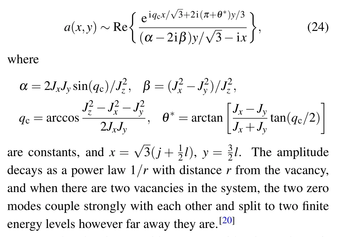
As an analog of the px+ipysuperconductor, the Majorana zero mode bound to a vacancy with aπflux in the Kitaev model under the[111]magnetic field may be solved in the continuum limit of the model as shown in Ref. [32]. We briefly recapture the calculation here and compare it with the results from the lattice model in the next subsection. Different from the p-wave superconductor, the Majorana mode in the Kitaev model in the continuum limit is a superposition of Fermionic modes in the two valleys instead of one.
A Majorana Fermion field in the Kitaev model in the[111]magnetic field may be expressed as

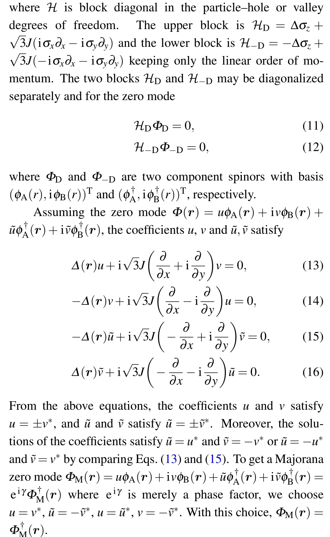
We then solve the MZM with aπflux bound to a vacancy. From the above relationship, we only need to solveu


3.2. Majorana zero modes in the lattice Kitaev model with a vacancy
The zero mode associated with a vacancy in the Kitaev model under the[111]magnetic field can also be obtained from the lattice Kitaev model. In this subsection,we show the similarities as well as the differences between the results from the continuum model and the lattice model.
The eigenstates of the lattice Kitaev model with a weak uniform [111] magnetic field and a vacancy can be obtained by directly solving the bilinear Hamiltonian Eq. (5) with an empty site.For the eigenstate with a vacancy site but flux-free,we setu〈ij〉α=1 for all the bonds. For the case with aπflux bound to the vacancy,we set thezbond operatorsu〈ij〉z=−1 along the half-infinite string in Fig. 1(a). In both cases, the Hamiltonian Eq.(5)becomes the following form:

whereAis a real anti-symmetric matrix and ˆcl,ˆcmare Majorana fermions. TheAmatrix then satisfies the following condition:

where ˆEis a diagonal and real matrix. For an eigenvectorUwith eigenenergyε, i.e., iAU=εU, one can get iAU*=−εU*from the above conditions. To obtain a Majorana eigenvector,Umust satisfyU= eiγU*,whereγis a real constant,soε=0,i.e.,the eigenenergy of a Majorana eigenmode must be zero for the lattice Kitaev Hamiltonian Eq.(5)with a vacancy.[24]
For the eigenstates with non-zero energy,the eigenvectorsUandU*with energy±εappear in pairs. For odd dimension of theAmatrix, there is at least one zero energy eigenmode.For even dimension ofA, the number of zero energy eigenmodes is even.
For a lattice withNunit cell and a single vacancy site,theAmatrix becomes a(2N −1)×(2N −1)matrix. For both the flux-free case and the case with aπflux threading through the vacancy plaquette, there is a Majorana zero mode. Whereas for the continuum model in the last section, the zero mode equations(13)-(16)have no solution in the flux free case. The zero mode in the lattice model in the flux free case is then due to the specific lattice configuration and is not robust.When the configuration of the vacancy changes, e.g., if the vacancy in the above model includes two neighboring sites,the Majorana zero mode disappears in the flux free case,which is verified in our numerics. However,the zero mode bound to theπflux is robust since it is induced by a topological defect and does not depend on the lattice configuration of the vacancy. Moreover,the zero modes in the two cases have different asymptotic behaviors,which we will study in details in the following.
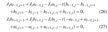
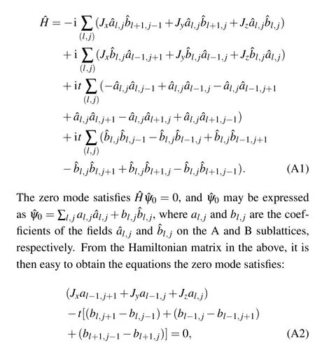
In the following we focus on the case with a single vacancy site in the lattice Kitaev model for simplicity and compare the Majorana zero modes in the flux free and flux threading cases. We only need to consider the vacancy on one of the two sublattices. The amplitudes of the zero mode for the vacancy on the other sublattice may be obtained by inversion symmetry.[19,20,24]Without loss of generality,we assume a vacancy on the B site in the following. We label the unit cell of the honeycomb lattice as in Fig.1(a). Each unit cell contains azbond. For the flux free case, the amplitudes of the vacancy induced zero mode satisfy the equations away from the vacancy as follows(shown in Appendix A):


whereal jandbl jare the amplitudes of the zero mode on the A and B sublattice of the unit cell(l,j),respectively,with the basis being the Majorana fermion ˆcon each site. The boundary condition near the vacancy is(a)Eq.(22)does not exist at(l,j)=(0,0); (b)for otherl,j=−1,0,1, Eqs.(22)and(23)are satisfied with the amplitudeb0,0=0.
Att= 0 and flux free, this zero mode was solved in Refs.[20,24,25]. It locates only on the opposite sublattice of the vacancy site since the A and B sublattices decouple in the zero mode in this case and the recursion factors of the amplitudes on the A and B sublattices are reciprocal, as shown in Appendix A.For the gapless Kitaev model and flux free case,the amplitude of the zero mode on the A sublattice away from the vacancy on a B site has the asymptotic form[24,25]
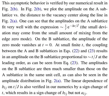
To solve the above problem,we consider the gapless Kitaev model with finitet. In this case, the finitetopens up a gap in the spinon bands with Chern number 1 or−1 and the vacancy induced zero mode decays exponentially in space.Different from thet=0 case,the A and B sublattices are now coupled together in the zero mode as shown in Eqs. (22) and(23)so the amplitudes on both sublattices are non-zero. However,the zero mode at finitetis no longer solvable analytically from Eqs.(22)and(23)and the boundary condition. We then solve the zero mode at finitetby numerically diagonalizing the corresponding bilinear Hamiltonian Eq. (19). The Majorana zero modeψwe obtained has Reψ=Imψ,i.e.,ψ†= eiπ/2ψ,in the flux free case. The phase factor eiπ/2may be gauged away by transformationψ →ψe−iπ/4, so we only need to study the real part ofψ. The distribution of the real part of the zero mode amplitude in the flux free case is shown in Fig.2(a)for the isotropic Kitaev model and a 120×120×2 lattice with a vacancy on the B sublattice in the center of the lattice. The parameters in the plot areJx=Jy=Jz=1,t=0.005. We only show the distribution of the zero mode around the central area of the vacancy since the influence from the edge mode in this area is negligible. Whereas near the edge of the lattice, the amplitude of the zero mode is dominated by the edge mode,which is not our focus in this subsection.

For the case with a flux threading the vacancy plaquette,the amplitudes of the zero mode also satisfy Eqs.(22)and(23)atl ̸=−1,0,1. However,the boundary condition the amplitudes match at the string connecting the vacancy site is different now. Since thezbond operator has the value−1 along the half-infinite string atl=0,Eqs.(22)and(23)become
forl=0,j ≥1. Besides,the boundary condition that Eq.(22)does not exist for(l,j)=(0,0)andb0,0=0 still needs to be satisfied.
Though the above equations for the zero mode with flux threading the vacancy plaquette are not solvable analytically even att=0,the boundary condition near the vacancy still results in nonzero amplitudes only on the A sublattice(vacancy on the B sublattice) att=0 as shown in Appendix A. At finitetwe solve the zero mode bound to the flux numerically and compare the asymptotic behavior of the amplitude with the analytical results obtained from the continuum model in the last section.

Fig.2. (a)The real part distribution of the amplitude of the zero mode for a 120×120×2 lattice with a flux free vacancy on a B site in the center and a weak uniform[111]magnetic field.The parameters are Jx=Jy=Jz=1 and t=0.005. The imaginary part of the amplitude is the same as the real part.Only the distribution of the central area including the vacancy is shown.(b)The real part of the amplitude on the A sublattice along the line in(a)as a function of the distance r to the vacancy center. The unit of r is the bond length of the hexagon. The amplitude ftis the curve uR e−kr, where k=∆/J˜,∆=6,and J˜=3J.
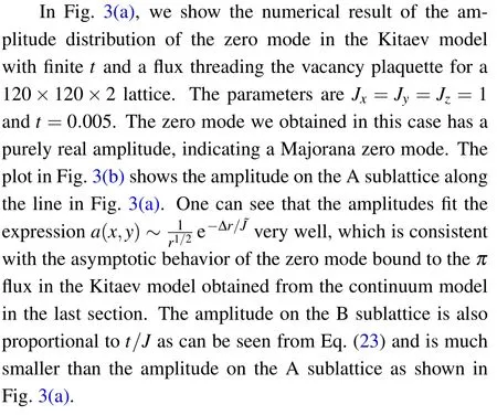

Fig. 3. (a) The distribution of the amplitude of the zero mode for a 120×120×2 Kitaev lattice with a flux threading the vacancy on a B site at the center of the lattice and a weak uniform[111]magnetic field.The parameters are Jx =Jy =Jz =1 and t =0.005. The amplitude of the zero mode is purely real. (b) The amplitude of the zero mode on the A sublattice along the line in (a) as a function of the distance to the vacancy center. The amplitude ftis the curve uR ~e−kr,where k=∆/J˜,∆=6?t,and J˜=J.
From above,we see that the Majorana zero modes in the flux free and flux threading cases have different asymptotic behaviors in the Kitaev model with finitet. As a comparison,we note that for the pure gapped Kitaev model with a single site vacancy,Ref.[20]shows that the amplitudes of the zero mode in both the flux free and flux threading cases are the same.The reason is because in this case the amplitude of the zero mode vanishes on one of the sublattices. The flux which flips the sign of the bond operatoru〈i j〉αalong the half-infinite string then does not affect the zero mode. On the other hand, the pure gapped Kitaev model has Chern number zero so a vortex does not bind an intrinsic Majorana zero mode. The zero mode in either the flux free or flux threading case with a single site vacancy is not robust and will disappear if the vacancy includes even number of sites.
3.3. Ground state with vortex binding to a vacancy in the lattice Kitaev model
The flux-threading and flux free cases in the last subsection belong to two independent eigensectors of the Hamiltonian Eq. (5). In this subsection, we show that for the Kitaev model in the weak[111]magnetic field,the ground state with a vacancy binds a flux in a certain regime of the magnetic field and thus results in a robust Majorana zero mode bound to the vacancy as shown in the last subsection.

Fig. 4. (a) Finite size scaling of the energy difference at WI =1 and WI =−1 of the Hamiltonian Eq. (6) with a vacancy. The system size is L×L×2,∆E=E0 −Eflux,where E0 is the ground state energy with WI =1 and Eflux is the ground state energy with WI =−1. (b)The energy difference ∆E extrapolating to the thermodynamic limit L →∞as a function of t.
It has been shown in Refs. [19,20] that the ground state of the isotropic gapless Kitaev model with a single vacancy binds aπflux and the ground state energy difference between the flux and flux-free cases is−0.027J. In Fig. 4, we show this energy difference at finitet, i.e., when a weak uniform[111]magnetic fieldhis applied.To remain in the perturbative regime so the bilinear Hamiltonian Eq.(5)is valid,we assumet~h3is small andh ≪1 (from the numerics in our previous work,t ≈2.7h3[26]). To minimize the finite size effect,we did finite size scaling of the energy difference between the flux and flux-free cases at each point oftin Fig. 4(a). The energy difference at eachtin Fig. 4(b) is the value that extrapolates to the thermodynamic limitL →∞. From the plot,we can see that the energy gain of the system with the flux threading the vacancy decreases with the increase of the magnetic fieldhand becomes negative at aroundt/J>0.004. We then see that for the isotropic Kitaev model in a uniform[111]magnetic field, at abouth/J<0.11, a single vacancy binds a flux in the ground state and a Majorana zero mode associated with it. This vortex bound Majorana zero mode decays exponentially with distance to the vacancy and is robust against local perturbations[21]and other Majorana zero modes farther away than the decay lengthξ~J/6t.[23]These Majorana zero modes may then have potential use in braiding in quantum computing.
4. Majorana zero modes induced by local polarization
In this section, we study a second type of defect in the Hamiltonian Eq. (5), i.e., a locally polarized spin in the uniform system, and the possible Majorana zero mode bound to such defect. The polarized spin is another type of topologically trivial spot and may be achieved and manipulated by a local magnetic field.
4.1. Model and method
For simplicity,we consider a local conical magnetic field applied to a single site on top of the system described by Hamiltonian Eq. (5), i.e., the Kitaev model with a perturbative uniform [111] magnetic field. The total Hamiltonian in the Majorana representation has the following form:

In the following,we study the evolution of the the above system with the increase of the local magnetic field and explore possible flux binding in the ground state upon local polarization and the Majorana zero mode associated with the flux.
With onlyHKandHh,the bond operator is still conserved,so does the flux in each hexagon plaquette. However,when a local magnetic field is applied on site 0 shown in Fig.1(c),the flux through the three hexagon plaquettes including the site 0 is not conserved though the total flux of these three plaquettes is conserved. We call the big plaquette including these three honeycomb plaquettes(the shaded area in Fig.(a))the impurity plaquette and call its flux operatorWIthe impurity flux.
We work in the flux sector that all the outer hexagons haveW=1.This corresponds to the ground state of the pure Kitaev model as well as the ground state of the Kitaev model with a vacancy at site 0. Since the impurity fluxWIis conserved,we deal with the two sectors withWI=+1 andWI=−1 separately. Note that for the pure Kitaev model, the ground state hasWI=+1,whereas for the Kitaev model with a vacancy at site 0,the ground state hasWI=−1.
When the local magnetic field is applied on site 0,only the three bond operators connected to site 0 are non-conserved.For the impurity flux free case, we may set all the other bond operatorsu〈ij〉α= ibαi bαjequal to 1. For the case withWI=−1, a string withuz=−1 connecting the impurity plaquette and the boundary of the system is introduced as shown in Fig. 1(a). The open boundary condition is applied. Under this convention, the local constraintDi=1 only needs to be imposed on sitei=0.
For convenience, we relabel the three nearest neighbor sites connected to site 0 asα=x,y,zas shown in Fig. 1(c),and the six next nearest neighbor sites connected to site 0 asαr,wherexr=1,2,yr=3,4,zr=5,6 are labeled in Fig.1(c)respectively.
The Kitaev Hamiltonian then becomes

We then use the mean field theory to study the local polarization process in the following. The applicability of the mean field theory has been tested in previous work on a[001]local magnetic field acting on the Kitaev model, where the mean field results agree very well with the exact numerical renormalization group results.[27]Actually the mean field theory is exact athloc→∞and is especially relevant at the locally polarized phase where the fluctuation of the bond operators connected to site 0 is highly suppressed. And this is the regime we are especially interested in in this work.
We decouple the quartic terms inHKandHhto quadratic terms by the mean field theory as follows:

4.2. Mean field results of the magnetization process
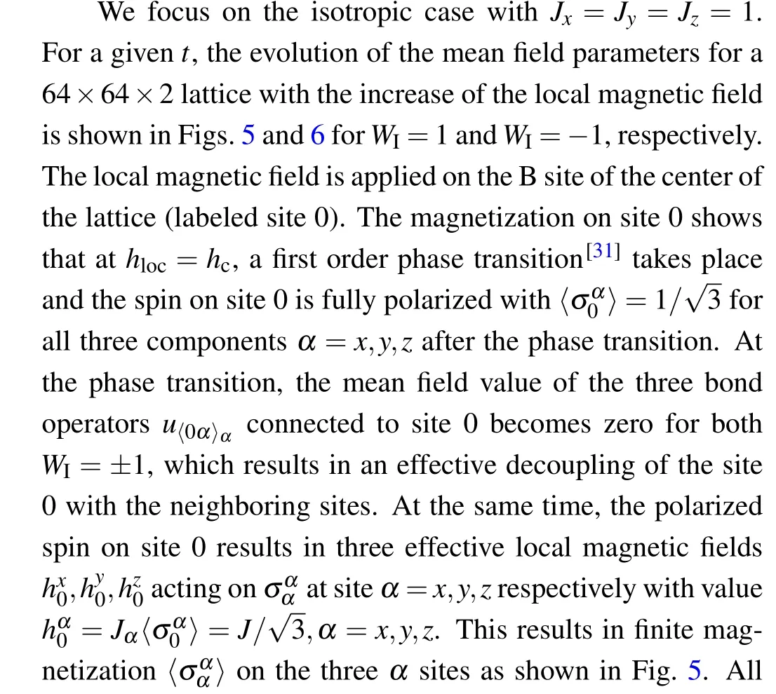


Fig. 5. The evolution of the mean field parameters as a function of the local magnetic field on site 0 in the impurity flux free case for a 64×64×2 lattice. The parameters Jx=Jy=Jz=1 and t=10−4. Upper: the three bond operators u〈0α〉,α=x,y,z connecting site 0 and site α. The mean field value of the three bond operators all goes to zero at the phase transition hloc=hc. Lower: the local magnetization on site 0 and sites x,y,z.After the phase transition at hc,the spin on site 0 is fully polarized and has〈σ0α 〉=1/3 for all three components α =x,y,z.
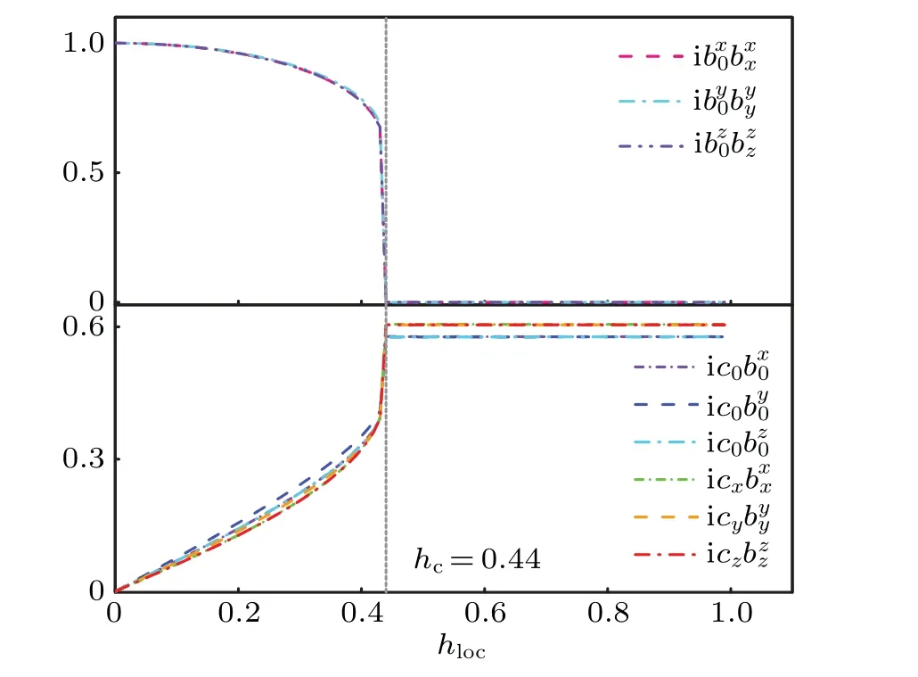
Fig.6. The evolution of the mean field parameters as a function of the local magnetic field on site 0 in the case with impurity flux WI=−1 for the same lattice in Fig.5. The legend is the same as that in Fig.5. The three bond operators u〈0α〉,α=x,y,z also go to zero after the phase transition at hc and the spin on site 0 is fully polarized with〈σ〉=1/for all three components α =x,y,z.
Figure 7 shows the energy difference of the two cases withWI=1 andWI=−1 as a function of the local magnetic field obtained from the mean field theory forJ=1,t=10−4and the lattice with size 64×64×2. We can see that the flux free caseWI=1 has lower energy in the local magnetic fieldhlocbefore the phase transition athloc=hc. However, after the phase transition,the state withWI=−1 has lower energy though the energy gain of the flux state in this case is much smaller than the case with only a vacancy in the last section.We then see that upon local polarization,the impurity plaquette binds a flux in the ground state at smallt.

Fig.7.The energy difference ∆E=E0 −Eflux between the impurity flux case and flux free case as a function of the local magnetic field from the mean field theory at Jx =Jy =Jz =1, t =0.0001 for a 64×64×2 lattice. Before the phase transition at hloc =hc =0.595, the flux free case has lower energy. After the phase transitions for both the WI=±1 cases,the flux state WI=−1 has lower energy,indicating a flux binding at the ground state after the polarization of the spin on site 0. Note that the transition field hc as well as ∆E in this plot is the corrected value after considering superheating of the first order phase transition so hc is slightly lower than the polarization field hc in Fig.5. See Ref.[27]for the correction procedure.
The flux threading the impurity plaquette at the ground state after phase transition athcresults in a Majorana zero mode at the ground state. We obtain a Majorana zero mode with purely imaginary amplitude. The distribution of the imaginary part of the amplitude is shown in Fig. 8 forJ=1,t= 10−4and a local magnetic field on a B site. Opposite to the vortex induced zero mode with a vacancy on site B in Fig.3,the amplitude of the zero mode on the A sublatticeal jis now much smaller than that on the B sublattice as shown in Fig. 8(a). This is because with the three effective local magnetic fields on the threeα=x,y,zsites after the polarization,the boundary condition of the zero mode near the site 0 is different from the case with only a vacancy on site 0. Att=0,the new boundary condition results in a zero mode with finite amplitudebijon the sublattice B but zero amplitudeai jon sublattice A,as shown in Appendix A.This is opposite to the case with only a vacancy on siteB. Note that the amplitudes of the three field ˆbααon the three A sitesα=x,y,zare still nonzero in this zero mode. For finite smallt,the coupling between the A and B sublattices in the zero mode equation results in a small amplitude on the A sublattice proportional to~t/J,as shown in Fig.8(a).
Fig.8.(a)The amplitude distribution of the Majorana zero mode bound to the flux after the polarization of a local spin on a B site. The parameters are Jx=Jy=Jz=1 and t=10−4.(b)Fitting curve of the amplitude on the B sublattice along the line in(a).

For the flux free case,due to the three effective local magnetic field, three Majorana fermion fields ˆbααenter the bilinear Hamiltonian in Eq. (35) and the dimension of the bilinear Hamiltonian matrix becomes even as(2N+2)×(2N+2).There is no Majorana zero mode after polarization in this case.This is verified in the spectrum we obtained numerically.
With the increase oft, however, the energy gain of the flux state after polarization of the local spin at site 0 becomes negative.As shown in Fig.9,att>4×10⁻⁴andJ=1,the extrapolation of ∆EtoL →∞becomes negative and the ground state of the polarized state remains to be the flux free stateWI=1 and there is no Majorana zero mode in the ground state after the polarization.

Fig.9. (a)Finite size scaling of the energy difference ∆E =E0 −Eflux between the impurity flux case and the flux free case after the local spin polarization on site 0 in both cases for parameters Jx=Jy=Jz=1 and t =10−4. Both E0 and Eflux are computed through the bilinear Hamiltonian Eq. (35). (b) The energy difference ∆E as a function of t. ∆E takes the value extrapolating to L →∞in(a).
In summary,we see that by polarizing a local spin in the Kitaev model with a weak uniform [111] magnetic field, the ground state of the system binds aπ-flux around the polarized spin which results in a Majorana zero mode that decays exponentially in space and is robust against local perturbation. At the same time,it may be easily manipulated by the local magnetic field in space. For these reasons, it may be a potential candidate for braiding in topological quantum computing.
5. Discussion and conclusions
As a comparison to the Majorana zero modes bound to local impurities in the above sections,we have a brief discussion of the edge Majorana modes for the above Kitaev model in the[111]magnetic field with a straight edge.


For the lattice Kitaev model Hamiltonian Eq.(6)with an infinite straight edge, however, the Hamiltonian has the form of Eq.(19)and from last section,the Majorna mode must have zero energy.The chiral edge modes with finite energy obtained from the continuum model are then not Majorana modes in the lattice model. Only the edge mode withky=0 is a Majorana mode in the lattice model which decays with the distance to the edge as~e−|∆x/J|.
In conclusions, we studied two types of defect induced Majorana zero modes in the ground state of the Kitaev model that decay exponentially in space and can be easily manipulated for braiding in quantum computing. In both approaches,we first applied a weak uniform [111] magnetic field on the Kitaev model which turns the Kitaev model to an effective px+ipysuperconductor of spinons. We then studied two specific defects, one is a vacancy in the Kitaev model, the other a polarized spin. Both defects correspond to a topologically trivial spot in the topologically non-trivial Kitaev system. We showed that both the single site vacancy and the fully polarized spin bind a vortex in the ground state at weak uniform[111]magnetic field. In both cases,the vortex results in a Majorana zero mode that decays exponentially in space and is robust against local non-magnetic perturbations and other Majorana zero modes far away.This is in contrast to the Majorana zero modes bound to pure gapless Kitaev model with vacancies. The Majorana zero modes we discussed in this work are then potential candidates for braiding in quantum computing.
Though the realization of the Kitaev model in real materials is still challenging,it is possible to be realized in a coldatom system.[29]At the same time, the fast development on single-site microscopy in optical lattices makes it promising to achieve and manipulate the Majorana zero mode we discussed in this work, especially through the locally polarized spin in the Kitaev model. In such case, a braiding procedure of Majorana zero modes may be performed according to the scheme discussed in a p-wave superconductor in Ref.[30].
Note After finishing writing this paper, we noticed Refs.[33-35]which discussed the effects of a local magnetic impurity coupling to the pure Kitaev model. These works mainly focus on the Kondo effect of the system and the impurity screened state of such system has some similarity with the system we study in this work but not exactly the same.
Appendix A
In this appendix,we show the derivation of the equations that the zero mode satisfies in the Kitaev model with a vacancy,and the results that witht=0 and a vacancy on a single B site as shown in Fig. 1(a), the amplitude of the zero mode is nonzero only on the A sublattice for both the flux free and flux-threading cases. Whereas for a vacancy on a single B site but with three local magnetic fieldshααon the neighboring sitesα=x,y,zas shown in Fig.1(c),the amplitude of the zero mode locates only on the B sublattice and the threeαsites att=0.
We first consider the case with only a vacacncy site without local magnetic field. The lattice configuration is shown in Fig.1(a)in the main text and the vacancy is on a B sublattice site. For simplicity,we label the Majorana fermion field ˆcon the sublattices A and B as ˆal,jand ˆbl,j,respectively in this appendix. In the flux free case,the Hamiltonian Eq.(5)can then be written as

These equations hold true everywhere except near the vacancy withl,j=−1,0,1. Near the vacancy,the zero mode satisfies the boundary condition in the main text,i.e.,(a)Eq.(A2)does not exist at(l,j)=(0,0);(b)for otherl,j=−1,0,1,Eqs.(A2)and(A3)are satisfied with the amplitudeb0,0=0.
Att=0,The above zero mode is not solvable analytically for finitet. But att=0,the zero mode may be solved by dividing the lattice to two partsl>1 andl<−1,and matching the boundary condition atl=0,1,−1. This zero mode was solved in Refs.[24,25]for the flux free case. We recapitulate the process here briefly and show some of the detailed derivation that is absent in the reference but also needed to study the case with local magnetic fields. For simplicity, we only consider the isotropic gapless caseJx=Jy=Jz=Jhere.
Att= 0, Eqs. (A2) and (A3) may be solved separately in thel> 0 andl<−1 regions. In these regions, the system has translation symmetry in thejdirection. By a Fourier transformational,j=∑k al(k)eik j,bl,j=∑k bl(k)eik j,k=2πm/N,m=1,2,...,N,one gets
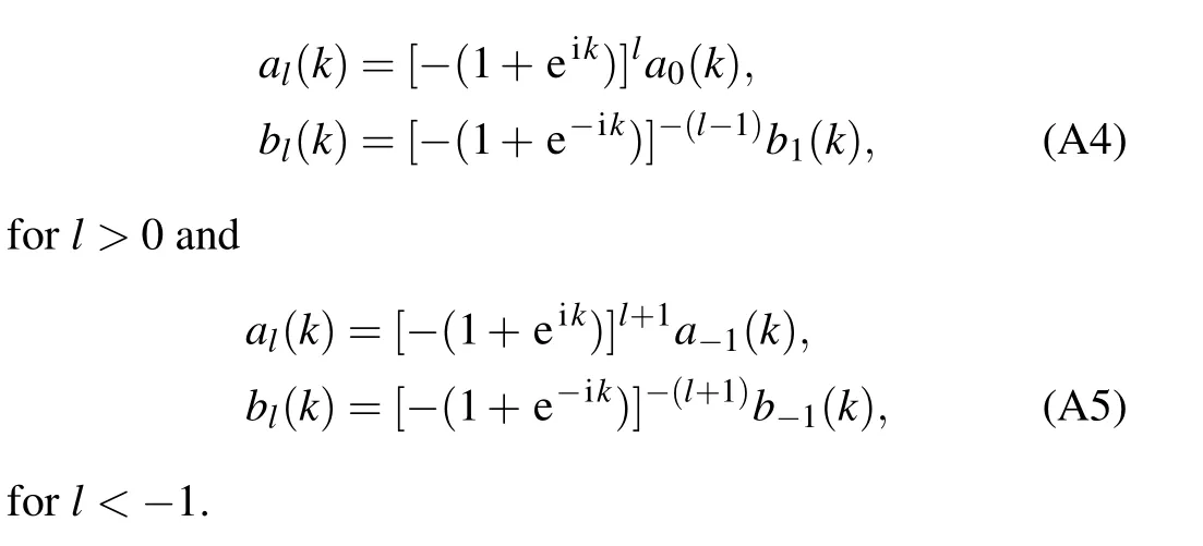
To have a decay solution, the recursion factors of bothal(k)andbl(k)need to have modulus less than one. From the above recursion relationships,one can see that the decay range ofkfor the coefficientsal(k)(orbl(k))atl>0 andl<−1 is complementary. And the decay range ofal(k)corresponds to the increase range ofbl(k) soal(k) andbl(k) cannot both be nonzero for a givenk.
Herea0(k),a−1(k),b1(k),b−1(k) are determined by matching the boundary condition. In the flux free case, the boundary condition foral,jisa−1,j+a−1,j+1+a0,j=0 except forj=0,i.e.,


These equations, together with the condition thatb−1(k) andb1(k)cannot both be nonzero for any givenk,result inb0(k)=b1(k)=b−1(k)=0 for allkwhich leads tobl(k)=0 for alll,i.e.,the coefficients of the zero mode on the B sublattice must be zero att=0.
The amplitude of the zero mode is then nonzero only on the A sublattice, i.e., the sublattice opposite to that of the vacancy site. One can then choosea0(k)=Θ[1−|f(k)|] and(1+eik)a−1(k)=Θ[|f(k)|−1], wheref(k)≡1+eik. The zero mode in this case may then be solved from the recursion relationship ofal(k)and the initial condition ofa0(k)anda−1(k) in the above, and then inverse Fourier transformation to the real space,as shown in Refs.[24,25].
We next consider the case with a flux threading the vacancy.
In this case,the recursion relationship foral(k)andbl(k)in Eqs.(A4)and(A5)still holds. However,the boundary condition atl=−1,0,1 becomes

Since the recursion relationship in Eqs. (A4) and (A5)still hold, the constraint thatb−1(k) andb1(k) cannot both be nonzero for a givenkstill works. Yet due to the flux, the boundary condition Eq.(A11)for the B sublattice is no longer true. However,it is easy to see that the solutionbl(k)=0 and sobij=0 still hold for the B sublattice. The amplitude of the zero mode then still locates only on the A sublattice in this case.
At last,we consider the case with a flux threading the vacancy and three local magnetic fieldshααacting on the three neighboringαsites as shown in Fig.1(c).
In this case, there are three local magnetic fields acting on the A sites of unit cell (0,0),(−1,0),(−1,1). The Majorana fields ˆcon these three sites then couple not only to the ˆcfield on the neighboring B sites, but also the ˆbααMajorana fermion on the same site. The recursion relationship atl>0 andl<−1 still holds. But the boundary condition the zero mode satisfies near the vacancy then becomes

猜你喜欢
中华养生保健(2022年10期)2022-05-23
海峡姐妹(2020年11期)2021-01-18
思维与智慧·上半月(2020年12期)2020-12-28
思维与智慧(2020年23期)2020-12-12
时代报告(2020年10期)2020-12-08
恋爱婚姻家庭·养生版(2020年3期)2020-04-13
文萃报·周二版(2020年9期)2020-04-10
妇女(2019年4期)2019-06-25
——博士跳楼
恋爱婚姻家庭(2016年28期)2016-10-11
恋爱婚姻家庭(2016年10期)2016-10-10

- Chinese Physics B的其它文章
- Numerical investigation on threading dislocation bending with InAs/GaAs quantum dots*
- Connes distance of 2D harmonic oscillators in quantum phase space*
- Effect of external electric field on the terahertz transmission characteristics of electrolyte solutions*
- Classical-field description of Bose-Einstein condensation of parallel light in a nonlinear optical cavity*
- Dense coding capacity in correlated noisy channels with weak measurement*
- Probability density and oscillating period of magnetopolaron in parabolic quantum dot in the presence of Rashba effect and temperature*