
Transient transition behaviors of fractional-order simplest chaotic circuit with bi-stable locally-active memristor and its ARM-based implementation
2021-12-22 06:40ZongLiYang杨宗立DongLiang梁栋DaWeiDing丁大为
Chinese Physics B 2021年12期
关键词:李浩
Zong-Li Yang(杨宗立) Dong Liang(梁栋) Da-Wei Ding(丁大为)
Yong-Bing Hu(胡永兵)1, and Hao Li(李浩)3
1School of Electronics and Information Engineering,Anhui University,Hefei 230601,China
2National Engineering Research Center for Agro-Ecological Big Data Analysis&Application,Anhui University,Hefei 230601,China
3State Grid Lu’an Electric Power Supply Company,Lu’an 237006,China
Keywords: fractional calculus,bi-stable locally-active memristor,transient transition behaviors,ARM implementation
1. Introduction
Chua has predicted that there is the fourth fundamental circuit element called memristor, which describes the relation between chargeqand magnetic fluxφ.[1]In 2008, HP(Hewlett Packard)Laboratory first fabricated a practical memristor physical device.[2]From then on, the research of the memristor received widespread attention in many fields of academia and industry. Due to its nonlinear and nonvolatile characteristics, memristors can be applied in many scenarios,such as neural networks,[3–5]memory storage,[6–8]chaotic circuit design[9–11]and secure communications.[12–14]
Researches show that the memristor has many types,and current popular memristors contain the HP memristors,[15–17]piecewise nonlinear memristors,[18–20]continuous nonlinear function memristors,[21–23]locally-active memristors,[24–26]and so on. Recently, the research of locally-active memristors has attracted wide attention because it has the capability of a nonlinear dynamical system to amplify infinitesimal energy fluctuations.[27–29]According to the principle of energy conservation, if a nonlinear dynamical system can produce and maintain oscillations, a locally-active element is essential. Oscillations occur only in locally-active regions.[30]As a novel memory device, the locally-active memristor is first proposed by Chua,[31]and it is considered to be the origin of complexity.[32]Chua proposed a corsage memristor with one pinched hysteresis loop and locally-active ranges, which was analyzed from complex frequency domain.[33]Oscillation of the circuit on the corsage memristor was analyzed via an application of the theory of local activity, edge of chaos and the Hopf-bifurcation.[34]A novel bi-stable nonvolatile locallyactive memristor model was introduced,and the dynamics and periodic oscillation were analyzed using the theory of local activity, pole-zero analysis of admittance functions, Hopf bifurcation and the edge of chaos.[35]Jinet al. proposed a novel locally-active memristor based on a voltage-controlled generic memristor, analyzed its characteristics and illustrated the concept of local activity via the DCV–Iloci of the memristor and nonvolatile memory via the power-off plot of the memristor.[36]Yinget al. proposed a nonvolatile locallyactive memristor, and the edge of chaos was observed using the method of the small-signal equivalent circuit.[37]Wanget al. proposed a locally-active memristor with two pinched hysteresis loops and four locally-active regions,and the effect of locally-active memristors on the complexity of systems was discussed.[38]
Fractional calculus is a generalization of the integer-order calculus,and it has the same historical memory characteristic as memristor with respect to time, therefore memristor and memristive system can be extended to fractional-order. Ivo Petr´aˇset al. firstly proposed the conception of the fractionalorder memristor.[39]Yuet al. demonstrated that fractionalorder system can describe memory effect better than integer order system in frequency domain.[40]Foudaet al. discussed the response of the fractional-order memristor under the DC and periodic signals.[41]A fractional-order HP TiO2memristor model was proposed, and the fingerprint analysis of the new model under periodic external excitation was made.[42]Wanget al. studied the properties of a fractional-order memristor, and the influences of parameters were analyzed and compared. Then the current–voltage characteristics of a simple series circuit that is composed of a fractional-order memristor and a capacitor were studied.[43]
Nowadays, there are many researches on locally-active memristor.[44–47]Fractional-order locally-active systems can generate more complex dynamic behaviors.However,there are few researches on the nonlinear characteristics of fractional-order locally-active memristor. Our objective is to propose a novel fractional-order continuous nonlinear bistable locally-active memristor model,and study its nonlinear characteristics and conclude that the fractional-order memristor is a bi-stable locally-active memristor in certain conditions.Then, we analyze the features of the fractional-order locallyactive memristor by time domain waveforms and pinched hysteresis loop at different frequencies, different amplitudes and different orders. In order to verify that the fractional-order memristor is locally-active, we design a fractional-order simplest circuit system using the designed memristor, a linear passive inductor and a linear passive capacitor in series. It is observed that the circuit can produce oscillation and its dynamical behavior is abundant. Particularly, the fractionalorder simplest nonlinear circuit using bi-stable locally-active memristor exhibits discontinuous coexisting phenomenon and rich transient transition phenomenon. Moreover, in order to verify the correctness of the theoretical analysis and numerical simulation, the fractional-order simplest chaotic system is implemented by ARM-based MCU. The contributions of this paper are listed as follows: (1) We design and analyze a fractional-order bi-stable locally-active memristor. (2) We build a fractional-order chaotic system based on the proposed memristor and discover its discontinuous coexisting dynamical behaviors and transient transition behaviors. (3)The proposed memristor and chaotic system are implemented digitally by ARM-based hardware.
The structure of this paper is organized as follows: Section 2 introduces the mathematical model of the fractionalorder bi-stable locally-active memristor and the power-off plot(POP)and DCV–Iloci are used to verify the nonvolatile and the locally-active characteristics. In Section 3, a fractionalorder nonlinear circuit using the proposed memristor is established, and the stability of the system is discussed. In Section 4,the nonlinear dynamics and transient transition behaviors of this system are revealed numerically using bifurcation diagrams, Lyapunov exponent spectrum, and phase portraits and so on. In Section 5,the circuit implement is carried out by ARM-based MCU in order to verify the validity of the numerical simulation results. Finally, some concluding remarks are given in the last short section.
2. Preliminaries
In this section,the mathematical definition of the Caputo fractional derivatives and Adomian decoposition method are introduced.
2.1. Fractional calculus
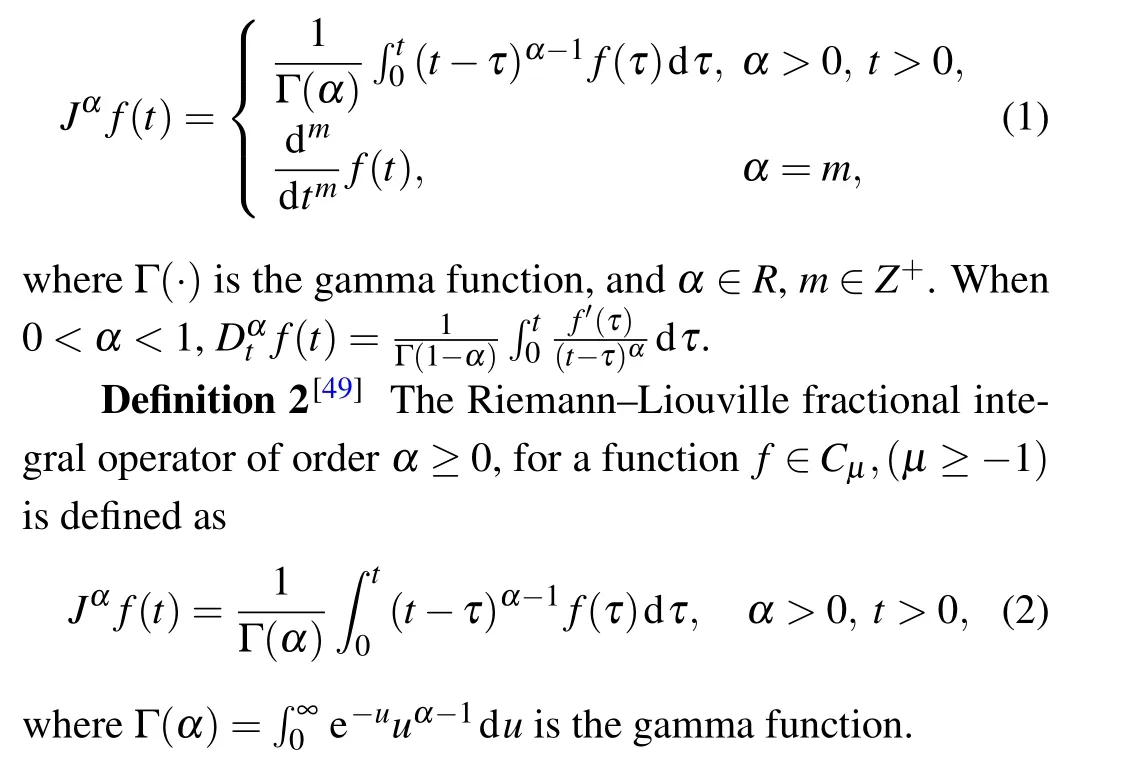
Definition 1[48]The Caputo fractional derivation definition of fractional-orderαis
2.2. Adomian decomposition method
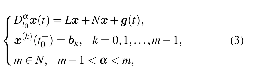
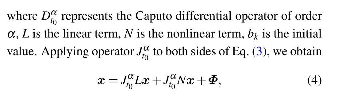
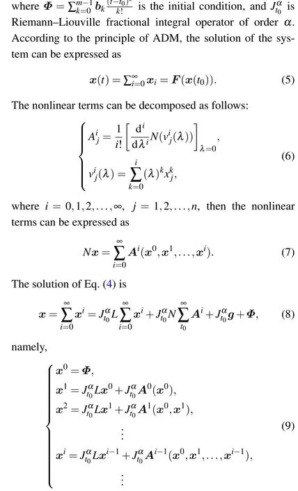
For a fractional-order chaotic systemDαt0x(t) =f(x(t)) +g(t), herex(t) = [x1(t),x2(t),...,xn(t)]Tare the state variables of the given function, andg(t) =[g1,g2,...,gn]Tare the constants for the autonomous system,and the functionfcan be divided into linear and nonlinear termsk
3. Bi-stable locally-active memristor
3.1. Memristor model
Based on Chua’s unfolding theorem,[50]a generic current-controlled memristor can be described by

wherevandiare the input and output of the memristor,respectively,xis the state variable, andg(·) andG(·) are functions related to a specific memristor.
A novel generic memristor model is proposed as follows:
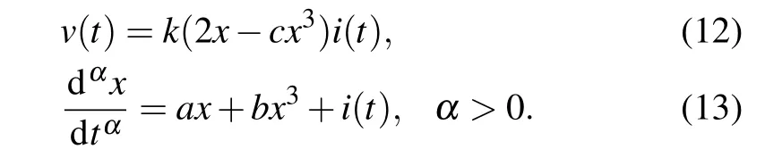
Based on Eqs. (12) and (13), when the unfolding parameters are set asa=4,b=−1,the POP of Eq.(13)with the arrowheads is shown in Fig. 1. Observing the trajectory of motion of the state variablex, we find that there are three intersections with thex-axis located atx1=−2,x2=0,x3=2. The dynamic route identifies that the equilibrium points−E1andE1are asymptotically stable, whereas the equilibrium pointE0is unstable, and the attraction domains of−E1andE1are(−∞,0)and(0,∞),respectively.

Fig.1. Power-off plot(POP)of Eq.(13).
3.2. Pinched hysteresis loops
A sinusoidal signal source with amplitudeAand frequenciesωis designed to drive the memristor. The dynamical trajectory displays one monostable or bi-stable pinched hysteresis loop as the amplitudeAand frequencyωof the sinusoidal signal source take different values.
Let the amplitudeA=4 V,α=0.9, and the frequencyωis changed. Whenω> 3.5 rad/s, the dynamical trajectory displays double coexisting pinched hysteresis loops as many initial valuesx0are situated on two sides of the origin.Letx0=1 andx0=−1,double coexisting pinched hysteresis loops can be obtained as shown in Figs. 2(a)–2(c). It can be found from Fig.2 that the double coexisting pinched hysteresis loops of the memristor are located in at least three quadrants.Forω>35 rad/s, although the dynamical trajectory displays double coexisting pinched hysteresis loops, the memristor is non-active.
Let the frequencyω=6 rad/s,α=0.9, and the amplitudeAis changed. WhenA<6.4 V,the dynamical trajectory displays one bi-stable pinched hysteresis loop as many initial valuesx0are situated on two sides of the origin. Letx0=1 andx0=−1, double coexisting pinched hysteresis loops can be obtained as shown in Figs.2(d)–2(f). The same conclusion can be obtained as above.
Let the amplitudeA=5 V,α=0.9,and the frequencyωis changed. When 1.4 rad/s≤ω<3.5 rad/s,the pinched hysteresis loops have a pinch-off point. When 0 ≤ω<1.4 rad/s,the pinched hysteresis loops have two pinch-off points,and all of the pinched hysteresis loops are symmetric abouti=0,the memristor is monostable memristor. The pinched hysteresis loops and corresponding time domain diagram are shown in Figs.3(a)–3(d).
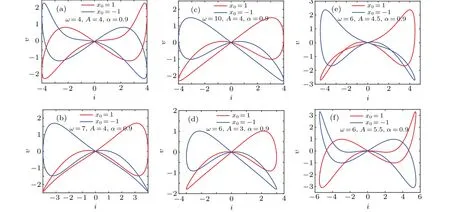
Fig. 2. Double coexisting pinched hysteresis loops when α =0.9, where red curves indicate initial value is x0 =1, blue curves indicate the initial value is x0=−1: (a)A=4 V,ω =4 rad/s,(b)A=4 V,ω =7 rad/s,(c)A=4 V,ω =10 rad/s,(d)A=3 V,ω =6 rad/s,(e)A=4.5 V,ω =6 rad/s,(f)A=5.5 V,ω =6 rad/s.

Fig.3. The time-domain wave and pinched hysteresis loops of monostable memristor: (a)the time-domain diagram when A=5 V,ω =2.1 rad/s,(b)the pinched hysteresis loops when A=5 V,ω =2.1 rad/s,(c)the time-domain diagram when A=5 V,ω =1.5 rad/s,(d)the pinched hysteresis loops when A=5 V, ω =1.5 rad/s, (e) the time-domain diagram when A=6.7 V, ω =3 rad/s, (f) the pinched hysteresis loops when A=6.7 V,ω =3 rad/s,(g)the time-domain diagram when A=8 V,ω =3 rad/s,(h)the pinched hysteresis loops when A=8 V,ω =3 rad/s.
In the same way, let the frequencyω=5 rad/s, and the amplitudeAis changed. WhenA>6 V,the pinched hysteresis loops have one pinch-off point. When 6.85 V≤A<10.5 V,the pinched hysteresis loop has two pinch-off points, and all of the pinched hysteresis loops are symmetric abouti=0,the memristor is monostable memristor. The pinched hysteresis loops and corresponding time domain diagram are shown in Figs.3(e)–3(h).
Let the amplitudeA=4 V,ω=5 rad/s, and the orderαis changed. When 0.787 ≤α<1, the pinched hysteresis loop has two pinch-off points. With the orderαincreasing,the non-origin pinch-off point moves from left to right until it disappears. Whenα<0.787,the pinched hysteresis loop has a pinch-off point of the origin,and it is symmetric abouti=0.The pinched hysteresis loops are shown in Fig.4.

Fig. 4. The pinched hysteresis loops when A=4, ω =5, where red curve indicates the order of α =0.9,green curve indicates the order of α =0.8,blue curve indicates the order of α =0.7.
3.3. DC V–I plots
DCV–Iplot is the Ohm’s law of the memristor, which can clearly show the intrinsic features of the memristor. Letx=X, dx/dt|x=X=0,Eq.(13)can be described as follow:

Solving Eq. (14) for the equilibrium point (X,I), a function between the stateXand the applied DC currentIcan be derived,and we have


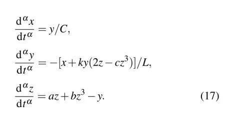
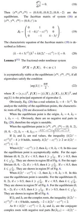
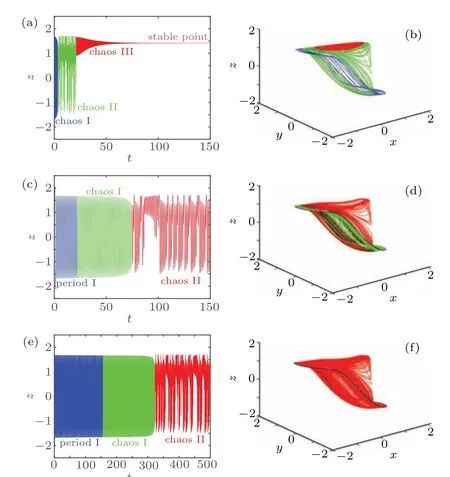
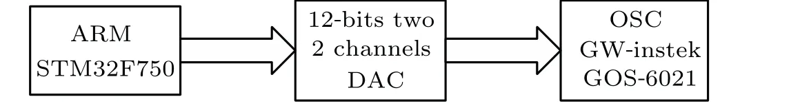
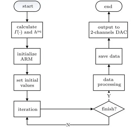
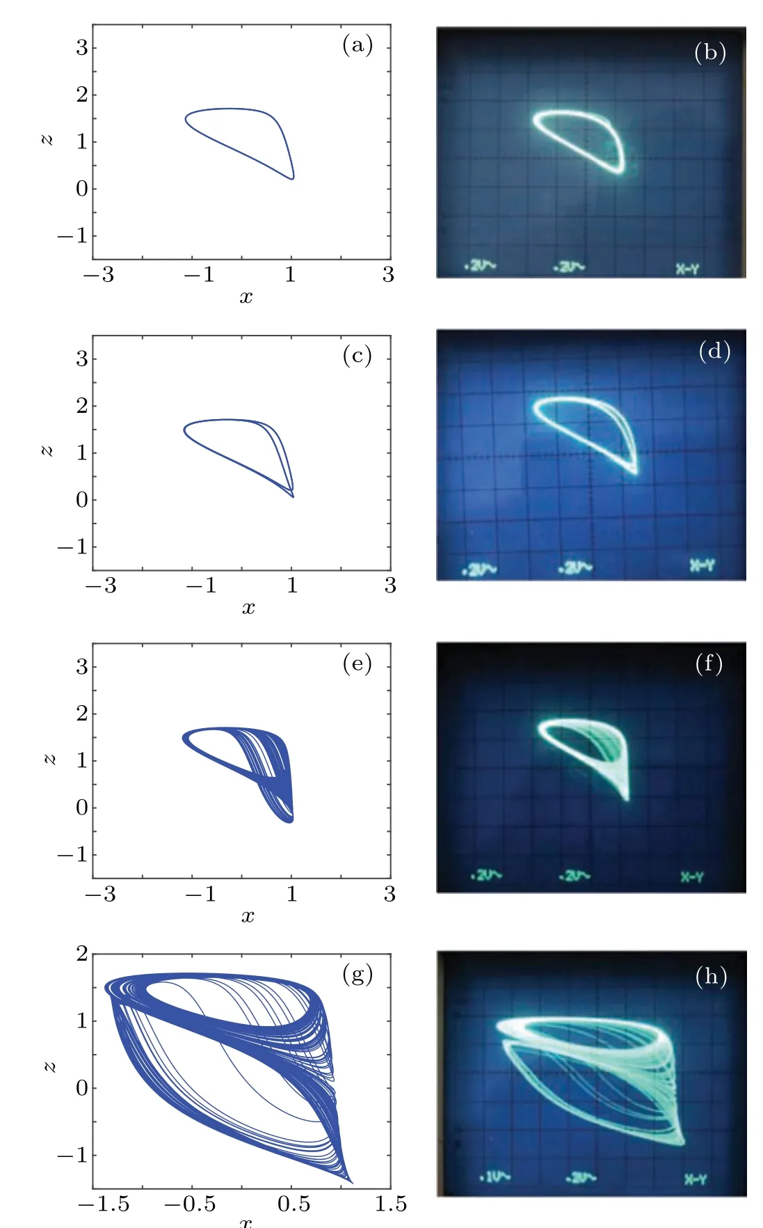
Fig.5. DC X–I and V–I loci. (a)The equilibrium state curve on the X–I plane for the DC current on interval −6 A Then settingk=1 and substituting Eq.(15)into Eq.(12),the DC voltageVcan be calculated as Based on Eqs. (15) and (16), when the parametercis set as 0.4, the DCX–IandV–Iplots of the memristor can be obtained, as shown in Figs. 5(a) and 5(b), respectively. When the parametercis set as different values,the DCV–Iplots are drawn as shown in Figs. 5(c) and 5(d). It can be seen from Fig.5 that the slopes of three parts of the DCV–Icurves are negative,hence the designed memristor is locally active. The well-known simplest chaotic system was presented by Chua.[51]The system contains three circuit elements,a resistance, an inductance and a memristor. When the memristor is replaced by a bi-stable locally-active memristor,a novel 3D autonomous fractional-order memristive chaotic system is given by The parameter values areC=1,L=1,a=4,b=−1.The state variables in terms of circuit variables arex(t)=vC(t)(voltage across capacitorC),y(t)=iL(t)(current through inductorL)andz(t)is the internal state of the bi-stable locallyactive memristor. From basic circuit theory,it is not possible to have an oscillation with three independent state variables if we use the non-active memristor. However,if we use a bi-stable locallyactive memristor in the circuit, the autonomous system can generate oscillation. To evaluate the equilibrium points,let The asymptotically stable regions and unstable regions in thek–cplane are separated by the curves ofk(2z∗−cz∗3)=2 andk(2z∗−cz∗3)=−2,which are shown as the red curves and blue curves in Fig.6,respectively. Fig.6. Asymptotically stable and unstable regions of the system(16)in the k–c plane. According to Eqs. (32)–(37), we can obtain the solutions of the proposed system,then analyze the dynamical characteristics of the system. Coexisting phase diagrams, coexisting bifurcation diagrams,basins of attractor and coexisting Lyapunov exponents are applied to analyze the dynamical behaviors of system(17). 4.3.1. Bifurcation analysis and Lyapunov exponents 4.3.1.1. Two-parameter bifurcation In order to show parameter-related dynamical behaviors of the proposed system, a two-parameter bifurcation diagram should first be computed. We know that there is a fractionalorder bi-stable memristor used in system (17), whena=4,c=0.5,α=0.8,two examples of two-parameter bifurcation diagrams for different initial conditions (x0,y0,z0)=(1,1,1)and (x0,y0,z0) = (−1,−1,−1) are shown in Figs. 7(a) and 7(b), respectively. The regions marked with different colors represent different attractor types and the navy blue regions imply the orbit tending to infinite. In addition, for different parameters, many classes of attractors cannot be completely distinguished, such as limit cycles with different periodicity and chaotic attractors with different topologies. The twoparameter bifurcation diagrams show rich dynamical behaviors and coexisting phenomenon in our system. Fig.7. Two-parameter bifurcation diagrams(a)in k–b plane for initial value(1, 1, 1), (b)in k–b plane for initial value(−1, −1, −1), (c)in α–b plane for initial value(1,1,1),(d)in α −k plane for initial value(1,1,1). In Fig.7(a),there are many regions marked with different colors,corresponding to the four different attractor types(navy blue region indicates the attractor tending to infinite),namely,cyan area, light area and yellow area indicate point attractor,limit cycle and chaos,respectively. Comparing Fig.7(b)with Fig. 7(a), it is easily seen that the two-parameter bifurcation diagram from system(17)is almost completely asymmetric. As shown in Fig. 7(c), there are three different attractor types,which are marked by three different colors,namely,the blue area indicates point attractors, light blue area indicates period attractors and the yellow area indicates chaotic attractors. In contrast, the period attractors have very small area marked by light blue,and the point attractors have biggest area marked by blue. In Fig. 7(d), there are three regions marked with different colors, corresponding to the three different attractor types. The blue area indicates point attractors,the light blue area indicates period attractors,and the yellow area indicates chaotic attractors.From Fig.7,stable point,periodic and chaotic areas can be easily identified. 4.3.1.2. Coexisting bifurcation Lyapunov exponents are considered as one of the most useful diagnostic tools for analyzing dynamical behaviors of nonlinear system,and coexisting bifurcation analysis can compare the characteristics of a nonlinear system in different initial values. The method of Ref.[54]is used to solve the Lyapunov exponents in this paper. Based on the two-parameter bifurcation diagram,we can trace the dynamics to compute a single-parameter bifurcation diagram, i.e.,b=1.5,b=−1.5 andk=0.5,k=−0.5. We choose two sets of different initial values (1, 1, 1) and (−1,−1,−1), and plot coexisting bifurcation diagrams ofxversusb,xversuskandzversusα. The corresponding bifurcation diagrams and Lyapunov exponents are shown in Figs.8–10,respectively. Fig.8. Bifurcation diagrams with respect to x and Lyapunov exponents.(a) k=0.5, xmax excited by two sets of initial value (1,1,1) (red) and initial value(−1,−1,−1)(blue),(b)k=0.5,coexisting bifurcation of xmax for initial value(1,1,1)(red)and initial value(−1,−1,−1)(blue),(c)k=0.5,Lyapunov exponents corresponding to(a),(d)k=0.5,coexisting Lyapunov exponents corresponding to(b), (e)k=−0.5, xmax excited by two sets of initial value(1,1,1)(red)and initial value(−1,−1, −1)(blue), (f)k=−0.5, coexisting bifurcation of xmax for initial value(1,1,1)(red)and initial value(−1,−1,−1)(blue),(g)k=−0.5,Lyapunov exponents corresponding to(e),(h)k=−0.5,coexisting Lyapunov exponents corresponding to(f). It is found from Fig.8 that system(17)occurs alternately the phenomenon of period and chaos with the increase of parameter. Whenk=0.5,b ∈[−8.2,−2.33], system (17) produces chaotic oscillation and period oscillation only in initial value (1, 1, 1). Whenk= 0.5,b ∈[−2.34,1.59], system (17) undergoes coexisting chaos and period-1 states, coexisting point attractor and period-1 states,coexisting point attractor and chaos states. Whenk=0.5,b ∈[1.6,13],the coexisting oscillation disappears and system(17)alternately occurs period and chaos oscillation only in initial value(−1,−1,−1).Whenk=−0.5,b ∈[−8.2,13],system(17)undergoes almost the same process ask=0.5, shown in Figs. 8(a), 8(b), 8(e),and 8(f). Symmetry reflects the beauty of harmony and unity.In general, if a system manifests a symmetric transformationT:(x,y,z)→(−x,−y,−z),it can be found that the system is invariant underT,and emerges dynamic behaviors in pairs. In contrast, our system does not satisfy the condition of a symmetric transformationT,we still find that the bifurcation plots are not perfectly symmetrical with respect tob-axis,xmax-axis and center. This indicates that system(17)with the proposed bi-stable locally-active memristor possesses the unique characteristics.The corresponding Lyapunov exponents are shown in Figs.8(c),8(d),8(g),and 8(h). Fig.9. Coexisting bifurcation diagrams with respect to x and Lyapunov exponents. (a)b=1.5,coexisting bifurcation of xmax for initial value(1,1,1)(red)and initial value(−1,−1,−1)(blue),(b)b=−1.5,coexisting bifurcation of xmax for initial value(1,1,1)(red)and initial value(−1,−1,−1)(blue),(c)b=1.5,Lyapunov exponents corresponding to(a),(d)b=−1.5,coexisting Lyapunov exponents corresponding to(b). It is found from Fig.9 that with the increase of parameterk, system (17) alternately occurs the phenomenon of periods and chaos. Whenb= 1.5,k ∈[−4,−0.5329], system (17)produces a stable point attractor only in initial value (1,1,1).Whenb=1.5,k ∈[−0.5328,−0.3], system (17) undergoes coexisting chaos and point attractor states,coexisting period-1 and point attractor states,whenk ∈[−0.3,0.3],the coexisting phenomenon disappears and system (17) undergoes chaos to period to chaos. Whenk ∈[0.3,0.5328], the coexisting phenomenon appears again, and system (17) undergoes a symmetrical process withk ∈[−0.5328,−0.3]. Whenb= 1.5,k ∈[0.5329,4], system (17) produces stable point attractor only in initial value (−1,−1,−1). Whenb=−1.5,k ∈[−0.5328,0.5328], system (17) undergoes coexisting chaos and point attractor states. Whenk ∈[−4,−0.5328]∪k ∈[0.5328,4], the coexisting phenomenon disappears and system (17) only appears stable point attractor. We find that the bifurcation plots are not perfectly symmetrical with respect tok-axis,xmax-axis and center. The corresponding Lyapunov exponents are shown in Figs.9(c)and 9(d). It is found from Fig. 10(a) that with the increase of parameterα,system(17)alternately occurs the phenomenon of stable point, periods and chaos. Whenb=−1.5,k= 0.5,α ∈[0.5,0.63], system (17) produces stable point attractor in all values. Whenb=−1.5,k= 0.5,α ∈(0.63,0.78],system (17) produces chaos oscillation in all values. Whenb=−1.5,k=0.5,α ∈(0.78,1],system(17)undergoes coexisting chaos and period states. The corresponding Lyapunov exponents are shown in Fig.10(b). Fig.10. Coexisting bifurcation diagrams with respect to z versus α and Lyapunov exponents. (a) k=0.5, b=−1.5, coexisting bifurcation of zmax for initial value(1,1,1)(red)and initial value(−1,−1,−1)(blue),(b)k=0.5,b=−1.5,Lyapunov exponents corresponding to(a). 4.3.2. Coexisting attractors and attraction basins If a nonlinear system with bi-stable memristor can produce oscillation, it must have coexisting attractors. Based on bifurcation plots in Figs. 7–10, we set parametersa=4,c=0.5,α=0.8,h=0.001 and change parametersbandk,then,we can draw phase diagrams as shown in Fig.11.We find that there are two kinds of chaotic attractors and two kinds of period-I cycles in the system,and called chaotic attractor I and chaotic attractor II, cycle I and cycle II. Figure 11(a) shows the coexistence of cycle I and chaotic attractor I.Figures 11(b)and 11(c)only show cycle I and attractor I,respectively. Figure 11(d) shows the coexistence of attractor I and pointer attractor. Figure 11(e)shows the coexistence of two pointer attractors in the system. Figure 11(f) shows the coexistence of chaotic attractor II and pointer attractor. Figure 11(g) shows the coexistence of cycle II and pointer attractor. Figure 11(h)shows the coexistence of cycle II and pointer attractor. From Fig. 11, we also can see the coexisting phenomenon of system(17)is intermittent. The different types of attractors coexist stably in the proposed simple chaotic system, their basins of attraction represent the states of the attractors in the initial state space.When we set parametersa=4,c=0.5,α=0.8,h=0.001 and change parametersb, we can draw basins of attraction as shown in Fig. 12. In Fig. 12, the basins of attraction of the point and chaos attractors of system(17)are indicated by blue and yellow, respectively. The light blue region indicates the attractor tending to infinite. Comparing Fig. 12(b) with Fig. 12(a), it is easily seen that the basins of attraction from system(17)have similar area shapes when the parameterbis set as 1 and−1. Fig. 11. Coexisting attractor, red curves indicate initial value of (1, 1,1), blue curves indicate the initial value of (−1, −1, −1); (a) k=0.5,b=−2.33, (b) k=0.5, b=−2, (c) k=0.5, b=−1.3, (d) k=0.5,b=−0.8,(e)k=0.5,b=0.4,(f)k=0.5,b=0.6,(g)k=0.5,b=1.2,(h)k=−1.5,b=1.15. Fig.12. Attractor basins for(a)b=1,(b)b=−1. Transient chaos and transient period are unique phenomenon in nonlinear systems with locally-active memristor.[55,56]This section will focus on the transient transition behaviors of the proposed system,and study the transient transition phenomena with changing parameters of the system and initial value. 4.4.1. Transient transition when parameter k changes To research the rich transient behaviors when the parameterkchanges, we firstly fix the parametersα=0.8,a=4,c=0.5,b=1.5 and initial value (1, 1, 1), then choose the parameterk ∈(0.01,0.51). Settingk= 0.06, the simulation timet ∈(0,300), the time-domain wave and phase diagram of the state variablezare shown in Figs. 13(a) and 12(b). Whent ∈(0,140), the time-domain wave is shown in the blue domain of Fig.13(a),in this time,LE1=0.0220,LE2=0.0073,LE3=−10.6775,so the system is chaos. Whent ∈(141,165),the time-domain wave is shown in the green domain of Fig. 13(a), the system displays an unstable chaotic state. Whent ∈(166,300), the system displays a period state, which is shown in the red domain of Fig.13(a).The corresponding phase diagram is shown in Fig. 13(b). Whenk= 0.13,t ∈(0,150), the system is chaotic state,which is shown in the blue domain of Fig.13(c),thent ∈(150,200), the system jumps from a chaotic state to another chaotic state, which is shown in the green domain of Fig.13(c). In this time,LE1=0.051,LE2=0.0062,LE3=−0.035,LE1+LE2+LE3>0,the system is an unstable chaotic state. Whent ∈(200,600),the system displays a clear three periods,which is shown in the red domain of Fig.13(c).The corresponding phase diagram is shown in Fig.13(d).With the parameterkincreasing, whenk=0.47,t ∈(0,220), the system is a single period state,which is shown in the blue domain of Fig. 13(e). Thent ∈(220,600), the system jumps from chaos I to chaos II state, which is shown in green and red domains of Fig.13(e). The corresponding phase diagram is shown in Fig.13(f). Fig. 13. The time-domain waveform and phase diagram of variable z, (a) k =0.06 time-domain waveform, (b) k =0.06 phase diagram,(c) k=0.15 time-domain waveform, (d) k=0.15 phase diagram, (e)k=0.47 time-domain waveform,(f)k=0.47 phase diagram. 4.4.2. Transient transition when parameter b changes When the parameterbchanges,we firstly fix the parametersα=0.8,a=4,c=0.5,k=0.5 and initial value(1,1,1),then vary the parameterb ∈(−8,1.59). Settingb=−5.4, the simulation timet ∈(0,600), the time-domain wave and phase diagram of the state variablezare shown in Figs.14(a)and 14(b).Whent ∈(0,60),the timedomain wave is shown in the blue domain of Fig.14(a),which indicates that the system is in cycle state,and the range of amplitude is(−1.5,1.5). Fig. 14. The time-domain waveform and phase diagram of variable z,(a)b=−5.4 time-domain waveform,(b)b=−5.4 phase diagram,(c)b=−0.73 time-domain waveform, (d) b=−0.73 phase diagram, (e)b=0.556 time-domain waveform,(f)b=0.556 phase diagram. Whent ∈(60,180), the time-domain wave is shown in the green domain of Fig.14(a),the system is in chaotic state.Whent ∈(180,600), the time-domain wave is shown in the red domain of Fig. 14(a). The corresponding phase diagram is shown in Fig. 14(b). Whenb=−0.73, the time-domain wave int ∈(0,50)is shown in the blue domain of Fig.14(c),and the system is in cycle state,the rang of amplitude is(1.1,1.5). Thent ∈(50,250), the time-domain wave is shown in the green domain of Fig. 14(c), the system is chaotic state.Whent ∈(250,600), the time-domain wave is shown in the red domain of Fig.14(c),which shows the system jumps from one chaotic state to another chaotic state. The corresponding phase diagram is shown in Fig.14(d).With the parameterbincreasing,whenb=0.556,t ∈(0,150),the time-domain wave is in a single period state,which is shown in the blue domain of Fig.14(e),thent ∈(150,450),the system jumps from one period to chaos I state,which is shown in the green domain of Fig.14(e). Whent ∈(450,600),the system changes from one chaotic state to another chaotic state, which is shown in the red domain of Fig.14(e). The corresponding phase diagram is shown in Fig.14(f). 4.4.3. Transient transition when parameter α changes To study the rich transient behavior when the parameterαchanges,we firstly fix the parametersa=4,c=0.5,k=0.5,b=1.5 and initial value(1,1,1),then choose the parametersα ∈(0.5,1). Fig. 15. The time-domain waveform and phase diagram of variable z, (a) α = 0.6 time-domain waveform, (b) α = 0.6 phase diagram,(c)α =0.77 time-domain waveform, (d)α =0.77 phase diagram, (e)α =0.79 time-domain waveform,(f)α =0.79 phase diagram. Settingα= 0.6, the simulation timet ∈(0,150), the time-domain wave and phase diagram of the state variablezare shown in Figs. 15(a) and 15(b). Whent ∈(0,5), the time-domain wave is shown in the blue domain of Fig.15(a),which indicates that the system is in a chaotic state. Whent ∈(5,25), the time-domain wave is shown in the green domain of Fig.15(a),and the system is in second type of chaotic state. Whent ∈(25,110),the time-domain wave is shown in the red domain of Fig. 15(a), the system is in third type of chaotic state. Whent ∈(110,150), the time-domain wave is shown in the pink domain of Fig. 15(a), and the system converges to a point. The corresponding phase diagram is shown in Fig.15(b). Whenα=0.77,att ∈(0,20),the time-domain wave is shown in the blue domain of Fig.15(c),and the system is in a single period state. Whent ∈(20,70),the time-domain wave is shown in the green domain of Fig.15(c),and the system is in a chaotic state. Thent ∈(70,150),the time-domain wave is shown in the red domain of Fig.15(c),and the system is in another chaotic state. The corresponding phase diagram is shown in Fig.15(d). With the parameterαincreasing,whenα=0.79,t ∈(0,150),the time-domain wave is shown in the blue domain of Fig.15(e),and the system is in a single period state. Whent ∈(150,320),the time-domain wave is shown in the green domain of Fig.15(e),and the system is in a chaotic state. Thent ∈(320,500), the time-domain wave is shown in the red domain of Fig. 15(e), and the system is in another chaotic state. The corresponding phase diagram is shown in Fig.15(f). It can be seen that system(17)transits from a state to another state, and finally stabilizes under the above parameters.There are two, three or four states from the beginning to the stable state,which is different from the transient transition behaviors reported in the literature. We implement the fractional-order bi-stable memristive simplest chaotic system on ARM platform. For hardware design, the block diagram of the working principle is shown in Fig. 16. In the experiments, the ARM-based MCU STM32F750 is employed. STM32F750 is a 32-bit ARMbased MCU running at 216 MHz with floating-point calculation unit. The processor comes with a 12-bit/8-bit dual channels digital-to-analog converter(DAC).Phase portraits of the system are captured randomly by an analog oscilloscope. The platform to implement the chaotic system (17) is shown in Fig.17. Fig.16. Block diagram for ARM implementation of a fractional-order chaotic system. Fig.17. Platform to implement a fractional-order chaotic system. The operational procedure of software design is shown in Fig. 18. After initializing ARM, we set the initial values(x0,y0,z0),parametersh,αand iteration number. Before iterative computation, we calculate all Γ(·) andhnα. Finally, all the data is transferred to DAC and shown in oscilloscope. Fig. 18. Flow chart for ARM implementation of a fractional-order chaotic system. Fig.19. Phase diagrams realized by ARM platform and recorded by the oscilloscope in x–z plane: (a)k=0.1,(b)k=0.15,(c)k=0.2,(d)k=0.45. We seta=4,c=0.5,b=1.5,α=0.8,h=0.01, initial values(x0,y0,z0)=(1,1,1), and change the parameterk.Phase portraits of the system are captured by the oscilloscope as shown in Fig.19. The experimental results qualify the simulation analysis. It indicates that the fractional-order bi-stable memristive simplest chaotic system is realized successfully on ARM platform. In this paper,a bi-stable locally-active memristor is firstly proposed, which has double coexisting pinched hysteresis loops and locally-active regions. Then, a fractional-order chaotic system based on the bi-stable locally-active memristor is explored, and the stability of equilibrium points of the system is analyzed. It is found that oscillations occur only within the locally-active region. By bifurcation analysis and Lyapunov exponent spectrum analysis, we find that the system has extremely rich dynamics, such as transient transition behaviors. Finally, the circuit simulation of the fractionalorder bi-stable locally-active memristive chaotic system is implemented on ARM-based MCU to verify the validity of the numerical simulation results.
4. Fractional-order bi-stable memristive system
4.1. The stability of the equilibria


4.2. Solution of the fractional-order bi-stable simplest memristive system

4.3. Analysis of complex dynamical behaviors


4.4. Transient transition


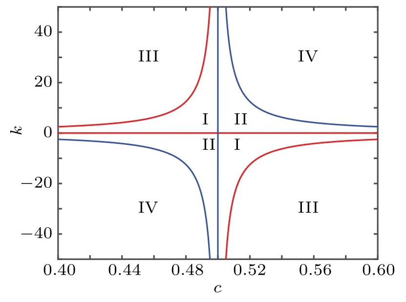
5. Implementation on ARM

6. Conclusion
猜你喜欢
基层中医药(2020年4期)2020-09-11
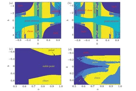
国画家(2017年5期)2017-10-16
军营文化天地(2017年7期)2017-09-25
时代文学·上半月(2017年5期)2017-05-15
时代文学·上半月(2017年5期)2017-05-15
当代工人(2017年2期)2017-03-27
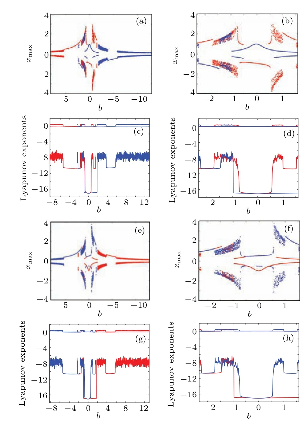
少林与太极(2016年4期)2016-06-16
中学生数理化·八年级数学人教版(2016年1期)2016-03-16
黄河黄土黄种人(2009年4期)2009-05-07

- Chinese Physics B的其它文章
- Modeling and dynamics of double Hindmarsh–Rose neuron with memristor-based magnetic coupling and time delay∗
- Cascade discrete memristive maps for enhancing chaos∗
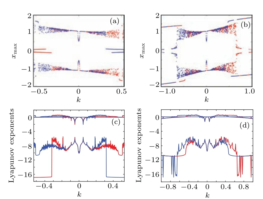
- A review on the design of ternary logic circuits∗
- Extended phase diagram of La1−xCaxMnO3 by interfacial engineering∗
- A double quantum dot defined by top gates in a single crystalline InSb nanosheet∗
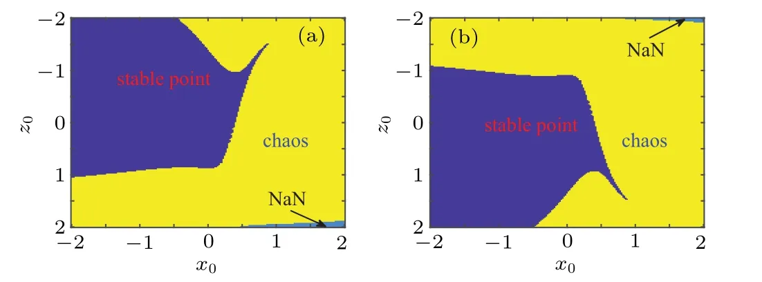
- Discontinuous and continuous transitions of collective behaviors in living systems∗