An Interior Bundle Method for Solving Equilibrium Problems

GAO Hui(高辉), GAO Shengzhe(高胜哲)

( School of Information Engineering, Dalian Ocean University, Dalian 116023, China)

Abstract: In this paper, by incorporating a logarithmic-quadratic function into the bundle method developed by Lemarchal and Wolfe (1975), we propose an interior bundle method for solving nonsmooth equilibrium problems.On one hand, the algorithm extends the bundle algorithm for equilibrium problems described by Nguyen et al.(2006) to our setting.The sequence generated by the proposed algorithm belongs to the interior of the set.On the other hand, we provide a natural extension of interior bundle methods to nonsmooth equilibrium problems.

Key words: Equilibrium problem; Interior bundle method; Logarithmic-quadratic function

1.Introduction

In this paper, we consider the nonsmooth equilibrium problem

where the continuous functionf:C×C →R, Csatisfy the following conditions:

(i) for allx ∈C, f(x,x)=0,f(x,·) is a convex function;

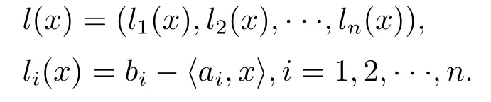
(ii) letCbe a polyhedral set with a nonempty interior given by

C:={x ∈Rn|Ax ≤b},

whereAanm×n(m ≥n) matrix with full rank, andb ∈Rm.

The equilibrium problem(1.1)plays an important role as a modelling tool in various fields.For example: variational inequalities, fixed point problems, optimization problems, saddle point problems,Nash equilibrium point problems in non-cooperative games,complementarity problems, in general, can be explored in [2-3].In recent years, many methods to solve the equilibrium problem have been much studied, such as the proximal point methods[4-5], the extragradient methods[6-8],and so on.Above all,they belong to the extension of the proximal point method in the final analysis.It is well known that the classical proximal point method is indeed a conceptual scheme for optimization, and the subproblems may be very hard to be solved when the objective function is nonsmooth.

For nonsmooth optimization problems, bundle methods are generally regarded as the most efficient and reliable.The main feature of this class of algorithmic schemes is the fact that replacing the objective function with a cutting-plane model to formulate a subproblem whose solution gives the next iteration and obtains the bundle elements.It was discussed in [9-10] since 1975.The bundle algorithm was then further developed and studied by Kiwiel[11-12].Later, the increasing interest is emphasized by a considerable number of papers on this topic.[13-16]However, only a few can be found for the equilibrium problem.To the best of our knowledge, the bundle algorithm to solve the equilibrium problem only was found in [1, 17].In [1], a bundle method using exact information for the equilibrium problem was studied.In [17], MENG et al.generalized bundle methods to inexact information for equilibrium problems.

In recent years, many researchers have replaced the quadratic regularization term in the algorithms by a distance-like function,some examples of which are: Bregman distances[7,18],φdivergence, and logarithmic-quadratic function[8,19-21].The main advantages of these extensions are that the sequences generated by the algorithms can stay naturally in the constraint set.Such a property cannot be ensured when using the usual squared Euclidean distance.In[19], the interior bundle algorithm withφ-divergence was designed for minimizing a convex function subject to nonnegative constraints.In [22], Auslender and Teboulle extended the algorithm with logarithmic-quadratic function to general linearly constrained convex minimization problems.Following a different approach, the interior bundle method developed in[23] uses a variable metric for nonsmooth convex symmetric cone programming.Then is it possible to extend the algorithm to the equilibrium problem and establish the corresponding convergence results?

In this paper, we consider the linearly constrained equilibrium problem.An interior bundle method for solving the equilibrium problem is proposed.Our approach extends the bundle algorithm for the equilibrium problem in[1].In addition,due to using the logarithmicquadratic function, the algorithm enforces the generated sequence to remain in the interior of the feasible set.This avoids solving constrained subproblems.Under mild conditions, the convergence of the algorithm is proved.What’s more,we provide some preliminary numerical results to demonstrate the algorithm.

This paper is organized as follows.Section 2 reviews some basic definitions and results required for this work.In Section 3, we present the interior bundle method for the problem(1.1).Section 4 examines the convergence properties of the algorithm.In Section 5, the Numerical experiments are given which illustrate the algorithm performances.Finally, we deduce our main work and the future possible research.

2.Preliminaries

In this section, we recall some definitions and basic results which will be used in the subsequent analysis.The Euclidean inner product in Rnis denoted by〈x,y〉=xTy, and the associated norm by‖·‖.

Letν ＞μ ＞0, and define

(see [21] for more details).By the definition ofφ, we define

We considerCis a polyhedral set with nonempty interior given by

C:={x ∈Rn|Ax ≤b},

whereAanm×n(m ≥n) matrix with full rank, andb ∈Rm.We denote byaithe rows of the matrixA, and for anyx,y ∈intC, we denote

ConsideringAis full rank, the inner product is defined by

with‖u‖A=‖Au‖=〈Au,Au〉moreover,

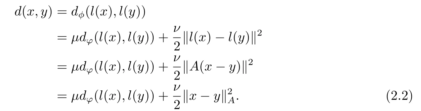
Lemma 2.1[20]Letd(x,y) be defined in (2.2), for allx,y ∈intC, then

(i)x →d(x,y) is strongly convex with modulusν, i.e.,

where∇1d(·,p) denotes the gradient map of the functiond(·,p) with respect to the first variable;

Lemma 2.2[19]LetF:C →R∪{+∞}be a closed proper convex function such that domF∩int∅, givenx ∈intCandck ＞0, then there exists the uniquey ∈intCsuch that

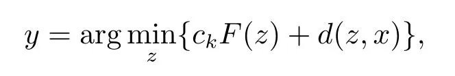
and

0∈ck∂F(y)+∇1d(y,x),

where∂F(y) denotes the subdifferential ofFaty.

Lemma 2.3[8]For allx,y,z ∈Rn,

3.Interior Bundle Methods

To establish the convergence of the interior bundle algorithms, we make the following assumptions for the nonsmooth equilibrium problem (1.1)

Assumption A

(i)C×C ⊂domf(·,·);

(ii) intC∅;

(iii) The subdifferential map∂f(xk,·) is bounded on the bounded subsets of intC.

Based on the proximal-like method in [24], the problem (1.1) can be reformulated as

The aggregate linearization

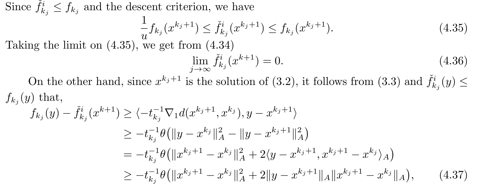
4.Convergence Analysis

Ⅰ Infinite null steps

This part will prove the convergence of the sequence when Algorithm 3.1 generates finitely many serious steps.We start with some preliminary results.For ally ∈intC,we define the following functions

We first prove the following preliminary result for the subsequent convergence.

Lemma 4.1For everyy ∈intC, then we have that

ProofBy the definition ofwe have

Sinced(·,xk) is strongly convex on intC, i.e., there existsν ＞0 such that, for ally ∈intC,

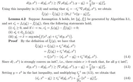
From this inequality in (4.4), it follows that

Summing up (4.7) and (4.8), we have that

i.e.,

We conclude from (4.10) and (4.11) that

Moreover,

hence

Summing up (4.15) and (4.16), we obtain

Since∇1d(xk,xk) = 0,we obtain that 0∈∂fk(xk), i.e.,xkis the solution of the equilibrium problem (1.1).

Ⅱ Infinite serious steps

This part is mainly concerned with the convergence of the sequence generated by infinitely serious steps.Firstly, we prove that the generated sequence{xk}is bounded and||xk+1-xk||→0.Secondly, we prove that every cluster point of the sequence{xk}k∈Nis a solution of problem (1.1).

In order to obtain the convergence of the algorithm, we need the following conditions.Assume that there existγ,c,d ＞0 and a nonnegative functiong:C×C →R,such that for anyx,y,z ∈C,

and

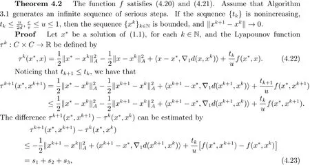
where

So,

Takingy=x*in (4.24), we have

and hence

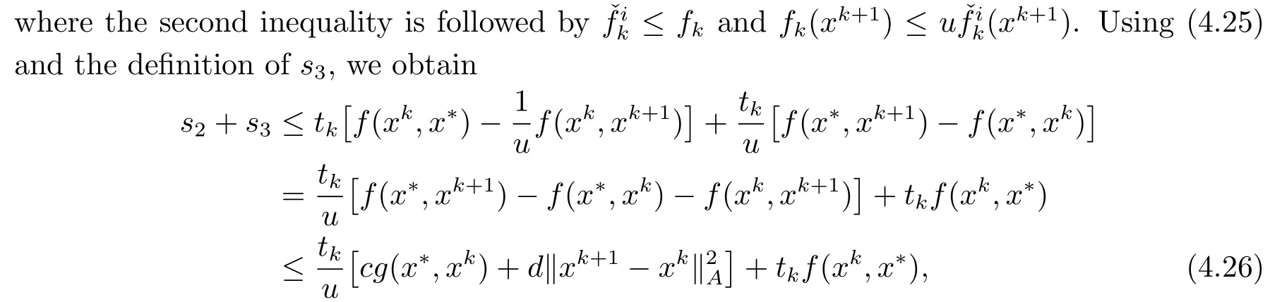
where the last inequality comes from the relation (4.21).Substituting (4.26) into (4.23), we have

Using (4.20) andx=x*,y=xk,f(x*,xk)＞0,we have

So (4.27) is

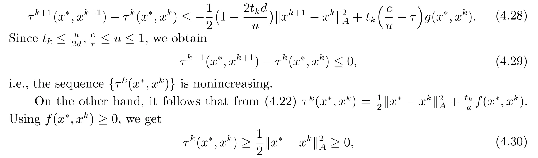
which means that{τk(x*,xk)}is bounded above zero.Using(4.29),the sequence{τk(x*,xk)}is convergent.Moreover, it follows from (4.30) that the sequence{xk}is bounded.Taking the limit on (4.28), we have that

Therefore,

Theorem 4.3Suppose that the conditions in Theorem 4.2 are satisfied, and Algorithm 3.1 generates an infinitely number of serious steps.Then every cluster point of{xk}is the solution of (1.1).

Becausefis continuous,

where the second inequality is obtained from Lemma 2.1,the equality is obtained from Lemma 2.3,and the last inequality is from the Cauchy-Schwarz inequality.Taking the limit on(4.37),we deduce from (4.32), (4.36)

5.Numerical Results

In this section, we propose some numerical experiments to test the effectiveness of Algorithm 3.1.All the optimization problems can be solved effectively by the function fmincon in Matlab Optimization Toolbox.All the programs are ran in Matlab (R2015b)PC Desktop Intel(R) Core(TM) i5-8250U CPU @ 1.60 GHz, RAM 8.00 GB.

Consider that the bifunctionf:C×C →R in (1.1) is expressed by

whereq ∈RnandP,Qare two matrices of ordernsuch thatQis symmetric positive semidefinite andQ-Pis symmetirc negative semidefinite.For the sake of simplicity, we consider that the feasible set isC=The matricesP,Qand the vectorqare the following ones :

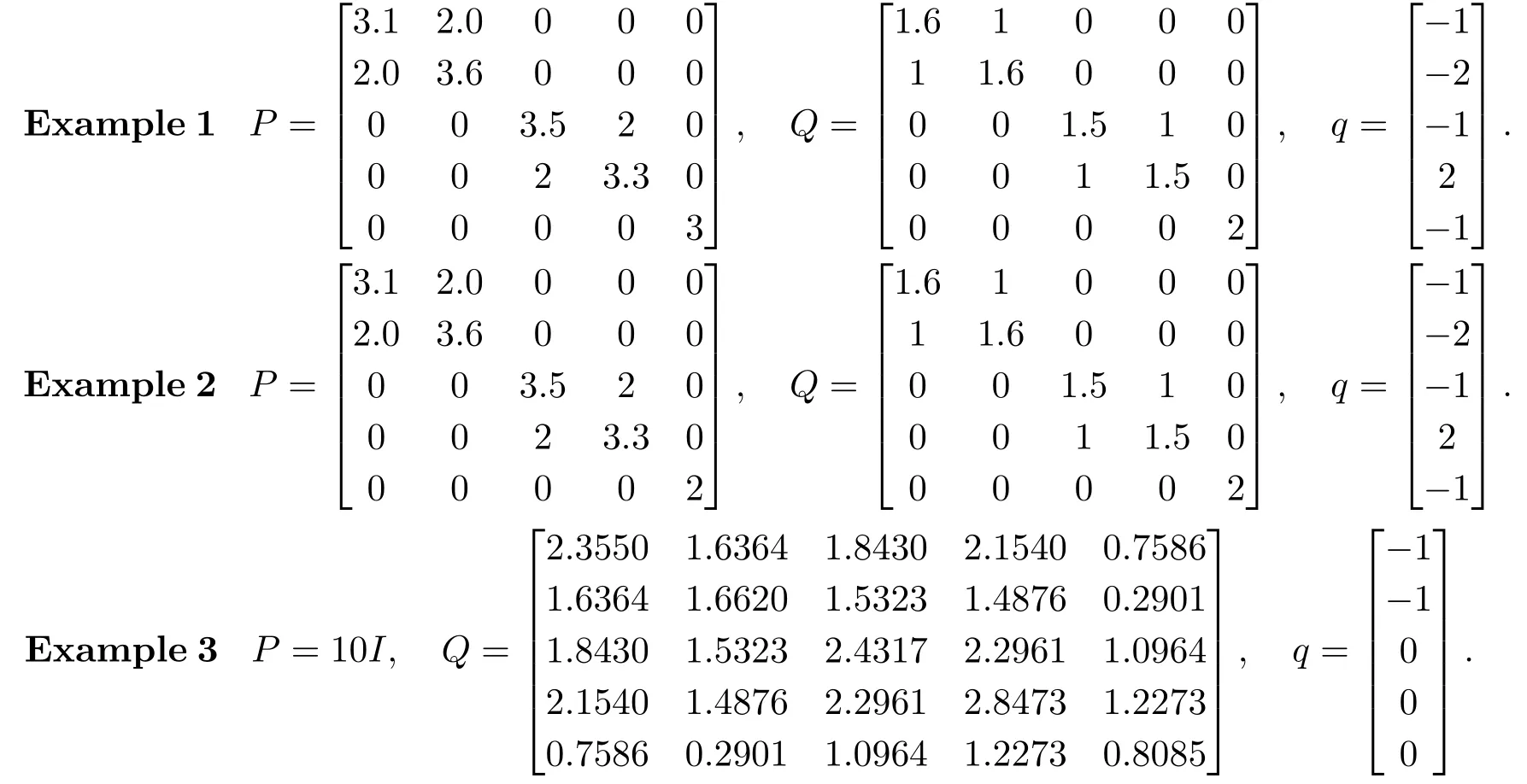
The functionφis chosen as follows:φ(t) =t-lnt-1 for allt ＞0.Letν ＞μ ＞0 be given fixed parameters, and define

To illustrate Algorithm 3.1, we introduce the numerical test of small size.The parameters are fixed toν= 7,μ= 1.The initial point isx0=y0= (1,1,1,1,1)Tfor the first two.For the third one, the initial point isx0=y0=(1,3,1,1,2)T.

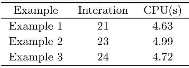
Tab.1 Numerical experimental results of Algorithm 3.1

6.Conclusions

In this paper,we propose an interior bundle algorithm for solving nonsmooth equilibrium problem.Under suitable conditions, we prove the convergence of the algorithm.Interesting features of the proposed method are as follows.Firstly, we extend theφ-divergence proximal distance of [21] to the equilibrium problem.Secondly, we present an interior bundle method to solve the equilibrium problem.As future work, it would be interesting to test our method for some numerical results or practical applications.It is also wanting to consider the case where the objective function is composite optimization problems.