
Robust SLAM localization method based on improved variational Bayesian filtering
2022-02-06 10:53ZhaiHongqiWangLihuiCaiTijingMengQian
Zhai Hongqi Wang Lihui Cai Tijing Meng Qian
(School of Instrument Science and Engineering, Southeast University, Nanjing 210096, China)(Key Laboratory of Micro-Inertial Instrument and Advanced Navigation Technology of Ministry of Education,Southeast University, Nanjing 210096, China)
Abstract:Aimed at the problem that the state estimation in the measurement update of the simultaneous localization and mapping (SLAM) method is incorrect or even not convergent because of the non-Gaussian measurement noise, outliers, or unknown and time-varying noise statistical characteristics, a robust SLAM method based on the improved variational Bayesian adaptive Kalman filtering (IVBAKF) is proposed. First, the measurement noise covariance is estimated using the variable Bayesian adaptive filtering algorithm. Then, the estimated covariance matrix is robustly processed through the weight function constructed in the form of a reweighted average. Finally, the system updates are iterated multiple times to further gradually correct the state estimation error. Furthermore, to observe features at different depths, a feature measurement model containing depth parameters is constructed. Experimental results show that when the measurement noise does not obey the Gaussian distribution and there are outliers in the measurement information, compared with the variational Bayesian adaptive SLAM method, the positioning accuracy of the proposed method is improved by 17.23%, 20.46%, and 17.76%, which has better applicability and robustness to environmental disturbance.
Key words:underwater navigation and positioning; non-Gaussian distribution; time-varying noise; variational Bayesian method; simultaneous localization and mapping (SLAM)
High-precision navigation and positioning technology is an important guarantee for underwater vehicles to successfully complete navigation detection and operation tasks[1-3]. In recent years, simultaneous localization and mapping (SLAM) technology has gradually become a research hotspot in the field of underwater navigation due to its advantages of realizing robot localization and real-time update environmental feature location only by continuously sensing the external environment information through sensors carried by itself without a prior map[4-6]. The extended Kalman filter (EKF)-SLAM algorithm has been widely used because of its rigorous mathematical theory, simple structure, and easy implementation, and it was first proposed by Smith et al[7]. In this method, spatial information is represented by a joint state vector containing the robot pose and environmental features, and the uncertainties of localization and feature estimation are expressed by the covariance matrix. Simultaneously, it is assumed that the noise obeys the Gaussian distribution. The EKF-SLAM algorithm is demonstrated in detail through theoretical derivation and experiments and optimized by Guivant et al[8-10]. The EKF framework was applied to the SLAM algorithm for underwater vehicles by Carpenter[11], and an environmental feature map was constructed, realizing the verification of the EKF-SLAM algorithm. The navigation system for underwater vehicles in partially structured environments, such as dams, ports, and docks, was described by Ribas et al.[12-13], and the feature information in the environment was extracted by a mechanical scanning imaging sonar. Meanwhile, the effectiveness of the EKF-SLAM algorithm is verified in an underwater environment at a depth of 600 m. Zhang et al.[14]proposed a consistency-constrained EKF-SLAM algorithm based on the idea of local consistency and applied it to the autonomous navigation of the C-Ranger AUV. Aimed at the problem of the azimuth variance accumulation error in the EKF-SLAM algorithm, the pose estimate is corrected using the absolute azimuth information given by an electronic compass, which improves the estimation accuracy of the EKF-SLAM algorithm[15].
However, the filtering accuracy of the standard EKF-SLAM algorithm depends on the accurate prior knowledge of noise statistics and Gaussian distribution assumption[16-17]. When an underwater vehicle operates, the noise statistical characteristics of the measurement sensors are usually unknown and time-varying due to the influence of complex hydrological environments, such as underwater organisms, salinity, and ocean currents, which will lead to a decrease in the filtering accuracy and may even cause filter divergence in severe cases[18-20]. Sarkka et al.[21]first proposed the combination of variable Bayesian learning and the Kalman filter method for state estimation of time-varying noise. Accordingly, more researchers began to pay attention to the study of variational Bayesian methods[22-25]. Aimed at the filtering problem of transfer alignment with an inaccurate measurement noise covariance matrix, a computationally efficient version of the existing variational adaptive Kalman filter is proposed[26], which facilitates the application of the variational adaptive Kalman filter to transfer alignment. To solve the problems of unknown state noise and uncertain measurement noise in coordinated underwater navigation, an adaptive EKF based on variable Bayesian for master-slave autonomous underwater vehicles is proposed by Sun et al[27]. Many uncertain factors in an underwater environment, such as abnormal clutters, reverberation interferences, marine noises, or mechanical vibrations of the power equipment inside the vehicle, will cause the noise characteristics of the measurement sensor under actual working conditions to have different degrees of non-Gaussian noise and cause the appearance of irregular outliers in measurement information. The generalized maximum likelihood estimation method based on Huber can effectively solve the non-Gaussian noise distribution problem. This method is an estimation technique combining the minimum and norms and has good robustness to the Gaussian distribution deviating from the assumption[28-29]. To handle the state and measurement outliers, a robust derivative-free algorithm named the outlier robust unscented Kalman filter was proposed[30]. Chang et al.[31]developed a robust version of the Kalman filter by introducing the Huber estimator into the recast linear regression to address process modeling errors in the linear system with rank deficient measurement models.
Therefore, to solve the problem that the state estimation is incorrect or does not converge in the measurement update phase of the SLAM algorithm caused by time-varying or the non-Gaussian distribution of the measurement noise and outliers in the measurement information, an adaptive robust SLAM localization method based on improved variational Bayesian filtering (IVBAKF-SLAM)is proposed in this paper. The main contributions are as follows:
1) The proposed algorithm uses the variational Bayesian filtering method to estimate the measurement noise covariance, then robustly processes the estimated covariance matrix utilizing the weight matrix, and finally performs multiple iterations on the system state update to gradually correct its estimation error, which further reduces the positioning error of the state estimation.
2) In the system model construction, we introduce depth information into the feature measurement model to fully observe the environmental features at different depths, which can better assist the navigation and positioning of underwater vehicles.
1 Proposed IVBAKF-SLAM Method
The basic idea of the feature-based EKF-SLAM algorithm is that the pose of underwater vehicles and features are augmented into the system state vector. At the same time, the system state is estimated using the filtering algorithm through the state prediction, measurement update, and state augmentation phases during the vehicle’s voyage, and the environment map containing the feature location estimation is constructed incrementally. In the measurement update phase, the standard EKF-SLAM algorithm assumes that the noise obeys the Gaussian distribution. However, due to the existence of various uncertain interference factors, such as signal disturbance in the practical application environment, the measurement system often has characteristics, such as non-Gaussian distribution or time-varying measurement noise, which may lead to incorrect state estimation or even non-convergence. Hence, a robust SLAM localization method based on the IVBAKF is proposed. In addition, to make full use of the feature information in the surrounding environment, the depth parameter of the feature is introduced into the measurement equation.
1.1 State prediction
Therefore, the augmented vector of the system state at timekcan be expressed as
(1)
where the north-east-down geographic coordinates are taken as the global coordinate system, and the origin of the vehicle coordinate system and the sensor coordinate system are assumed to coincide.
(2)
The corresponding covariance matrix can be expressed as[34-35]
(3)
wherePk-1expresses the covariance matrix of the system state at timek-1;Pδ,k-1denotes the covariance matrix corresponding to the state change at timek-1; andJk|k-1andUδ,k-1are the Jacobian matrices of the nonlinear model function with respect to the system state vector and state change, respectively. They can be expressed as
(4)
(5)
whereJvandUvcan be obtained by
(6)
(7)
1.2 Measurement update
During the navigation process, the environmental information could be obtained using sensing sensors, such as sonar, and the feature information could be extracted after preprocessing the obtained data. Then, the data association algorithm is used to judge whether the currently observed feature points match the existing features in the system state vector. If the currently observed feature is the existing feature in the state vector, the difference between the predicted value and measured value of the feature is used to update the vehicle pose and the position of the feature through the EKF method. However, when the measurement noise is time-varying or has a non-Gaussian distribution, the state estimation of the SLAM localization method based on the standard EKF algorithm may be incorrect or not convergent. Therefore, a robust IVBAKF method is proposed in the measurement update phase. Meanwhile, the measurement model containing the depth information of features is constructed to observe more features of different heights. The pressure sensor is used to measure the depth of the underwater vehicle. The data association method selected in this paper is the nearest-neighbor data association algorithm[36].
First, the relationship between the feature in the vehicle coordinate system and that in the global coordinate system is shown in Fig. 1.XgYgZgrepresents the global coordinate system, andXvYvZvrepresents the vehicle coordinate system. The asterisk denotes the vehicle, the circle denotes the feature,lidenotes the coordinates of the feature in the global coordinate system.ρirepresents the distance of thei-th feature observed in the vehicle coordinate system.αiis the angle between the projection of thei-th feature on the plane of the vehicle coordinate system and theXvdirection, andβiis the pitch angle of thei-th feature in the vehicle coordinate system.

Fig.1 Feature description in the global coordinate system and vehicle coordinate system
Therefore, the feature measurement model and depth measurement model can be expressed as
(8)
(9)
Therefore, the sensor measurement model can be expressed as
(10)
Then, the measurement equation can be abbreviated as the following discrete form:
(11)
wherezkrepresents the observation vector at timekandwkexpresses the measurement noise.

(12)
whereHkdenotes the Jacobian matrix of the measurement function and can be obtained by
(13)
where
Therefore, the system state model can be expressed as
(14)

(15)
whereμandηare the probability density distribution parameters of inverse gamma, and they can be obtained by
μk,i=μk-1,i+0.5
(16)
(17)
wherei=1,2,…,danddis the dimension of the measurement vector, the value of 0.5 can be determined by Ref.[21], and the subscriptiirepresents the diagonal element in the matrix.
Here, we define variablesTk,mk,Gk, andξkas follows:
(18)
(19)
(20)
(21)
Substituting Eqs.(18) to (21) into Eq. (14), it can be expressed as
mk=GkXk+ξk
(22)
Based on the generalized maximum likelihood estimation method, the corresponding iterative convergence solution can be expressed as
(23)
where the superscriptjrepresents the number of iterations, and the initialization value can be given by
(24)
From the valueΨcorresponding to the final convergent state, the corresponding state error covariance matrix can be obtained by
(25)
whereΨdenotes the weight function and can be given by
(26)
whereγis the regulatory factor andek,iexpresses the normalized residual of thei-th dimension.
Due to the special structure of the matrixGk, the state estimation process is further transformed into a more general form by applying the matrix inverse lemma. First, the weight matrixΨis divided into blocks, andΨxandΨyrepresent the state prediction residual and measurement prediction residual, respectively.
(27)
where0m×ndenotes them×nzero-valued matrix.
After derivation, the prediction covariance and measurement covariance matrix can be expressed as
(28)
(29)
Consequently, the estimated value of the system state and corresponding covariance matrix can be obtained by
(30)
(31)
(32)
1.3 State augmentation
If the currently observed feature is a new feature, it is integrated into the system state vector through the state augmentation process to realize incremental map construction. First, the current observation value is converted to the feature position in the Cartesian coordinate system through the following equation:
(33)
Then, it is augmented to the system state vector, and the expanded state function can be expressed as
(34)
The corresponding covariance matrix can be expressed as
(35)
(36)
wherePv,Pm, andPvmare the covariance matrices of the vehicle, map, and between the vehicle and map, respectively.
(37)
(38)
(39)
Consequently, the covariance matrix can be obtained by
(40)
Therefore, the newly observed features are expanded into the state vector through Eqs. (33) to (40), thereby realizing the expansion and construction of the map.
2 Experiments
To evaluate the effectiveness of the proposed IVBAKF-SLAM algorithm, we design three groups of experiments and compare them with EKF-SLAM and VBAKF-SLAM. The SLAM algorithm simulator used is based on the SLAM model provided by the Australian Centre for Field Robotics and is adjusted according to the kinematics model designed in this study. The experiments are carried out under the condition of known data association, which can eliminate the influence of incorrect data association on the filter estimation performance.
When an underwater vehicle sails, 28 environmental features are randomly distributed around the trajectory (assuming that these features remain stationary). The initial pose is {0,0,0,0°}, the velocity is 3 m/s, and the control frequency is 40 Hz. The observation distance of the sensor is 30 m, and the output frequency is 5 Hz. The three algorithms are performed in 30 Monte Carlo trials, and the average value is taken as the statistical result.
To verify the feasibility of the proposed method, the first set of experiments is set up. The observation noise is set toσρ=0.1 m,σα=1°,σβ=1°,σd=0.1 m, and the process noise is set toσv=0.1 m/s,σφ=2°. The comparison between the estimation trajectories for the three algorithms (i.e., EKF-SLAM, VBAKF-SLAM, and IVBAKF-SLAM algorithms) and the real trajectory is shown in Fig. 2. The position curves estimated by the three methods can basically follow the real trajectory, and the accuracy of the estimated trajectory based on the IVBAKF-SLAM algorithm is slightly better than those of the other two methods.
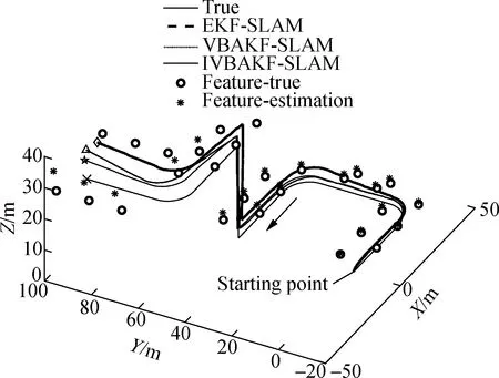
Fig.2 Trajectory comparison for the three methods in Experiment 1
To clearly describe the positioning accuracy of the three algorithms, the root mean square (RMS) errorξRkand average RMS (ARMS) errorξRkof the vehicle pose are introduced as evaluation indicators[37], which are defined as
(41)
(42)
Similarly, the RMS errorξLikand ARMS error avg(ξLik) of thei-th feature position are defined as
(43)
(44)
Therefore, the RMS value of the pose estimation error for the three methods can be calculated according to Eq. (41), as shown in Fig. 3. The positioning accuracy based on the IVBAKF-SLAM method is better than that of the VBAKF-SLAM and EKF-SLAM algorithms, regardless of whether it is the RMS error of the position estimation or that of the heading angle.
(a)
To quantitatively describe the filtering performance of the three methods, the ARMS value of the estimation error is calculated according to the definition of the average RMS error in Eqs. (42) and (44), as shown in Tab.1.
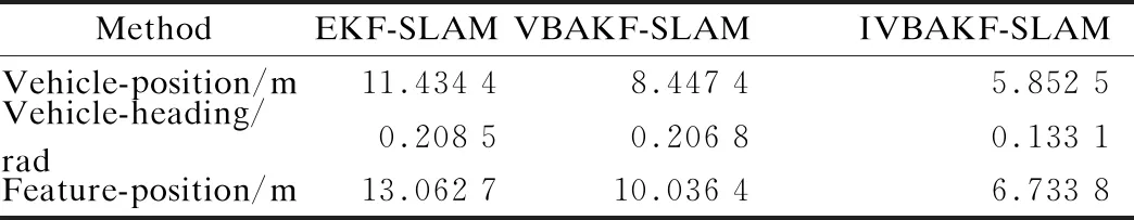
Tab.1 ARMS for the three methods in Experiment 1
In Tab.1, the ARMS of the position estimation from the IVBAKF-SLAM algorithm is 5.852 5 m, that of the heading estimation is 0.133 1 rad, and that of the feature estimation is 6.733 8 m. Compared with the EKF-SLAM and VBAKF-SLAM algorithms, the filtering performance based on the IVBAKF-SLAM method is relatively optimal.
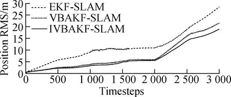
The second group of experiments is set up to evaluate the effectiveness of the proposed method when the measurement noise is time-varying. Here, the process noise is consistent with that in Experiment 1. The observation noise is set to 82Rduring 1 000 to 1 600 timesteps, set to 52Rduring the 2 000 to 2 600 timesteps, and set toRin other timesteps.R=diag(σ2) is the same as that in Experiment 1. Fig. 4 shows the RMS error of the pose estimation for the three methods. In Fig. 4, the RMS error of the position estimation and that of the heading angle estimation based on the IVBAKF-SLAM algorithm are relatively smaller than those of the other two methods.
(a)
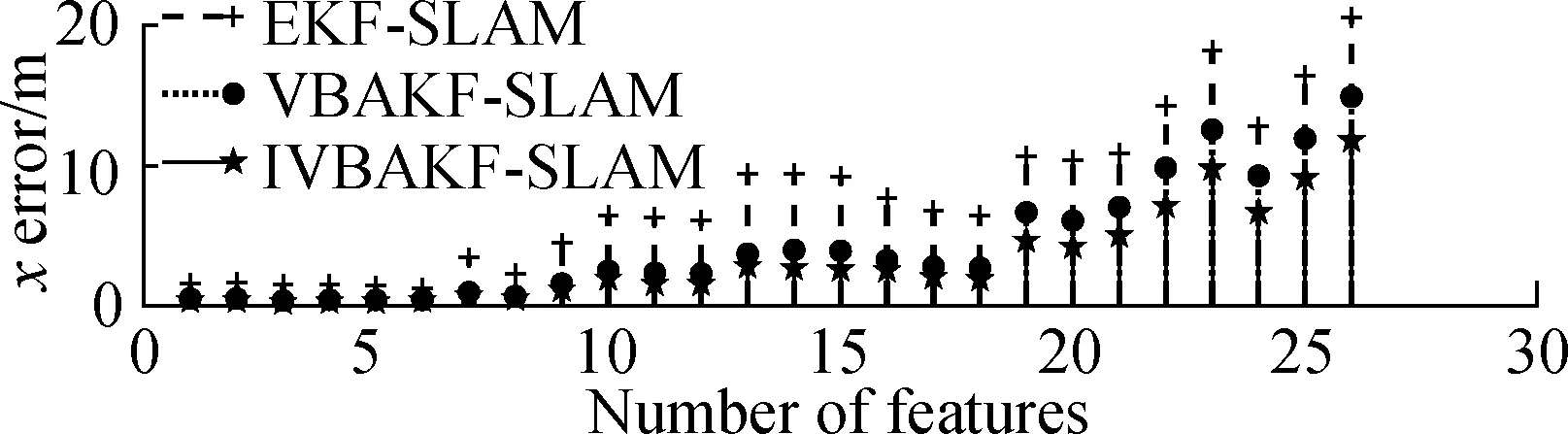
The estimation errors for the observed features are shown in Fig.5. The cyan curve marked with a plus sign expresses the estimated feature error based on the EKF-SLAM algorithm, and the point where each marked symbol is located represents thei-th observed feature. The estimation error curve of the VBAKF-SLAM algorithm is indicated by the dotted line marked with a circle, and that of the IVBAKF-SLAM algorithm is represented by the dotted line with a pentagram.
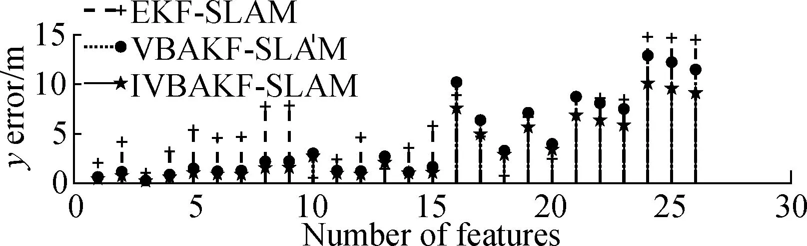
(b)
To compare the RMS errors of the position estimation for the three methods, the ARMS values of the vehicle and features observed in Experiment 2 are shown in Fig. 6. The ARMS-vehicle and ARMS-feature of the IVBAKF-SLAM algorithm are the lowest, and the EKF-SLAM has the maximum ARMS errors.
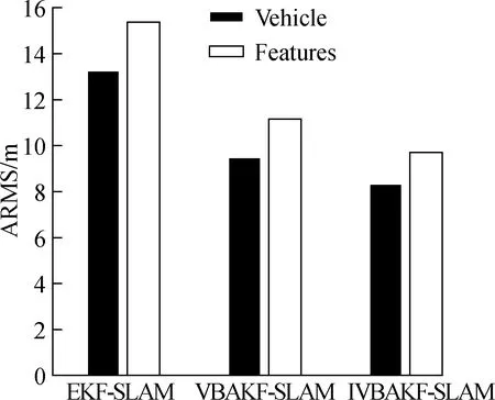
Fig.6 Comparison of the ARMS of the vehicle and features observed in Experiment 2
To verify the effectiveness of the proposed method when the thick-tail distribution exists in the measurement noise and there are outliers in the measurement information, the third group of experiments is set up. Similarly, the process noise is consistent with that in Experiment 1, and the measurement noise obeys the mixed Gaussian distribution in the following equation, where a 90% probability obeys the Gaussian distribution with a mean of 0 and variance matrix ofRand a 10% probability follows a Gaussian distribution with a mean of 0 and variance matrix of 100R.
(45)
whereR=diag(σ2) andσ=[0.1 1 1 0.1] are the same as those in Experiment 1. Meanwhile, an outlier is added to the measurement information every 200 time-step during the 500 to2 500 time-step. The measurement at the other timesteps is normal. The experiment results are shown in Figs. 7 to 9.
Fig.7 shows the comparison of the estimation trajectory for the three algorithms. The trajectory estimated by the EKF-SLAM method seriously deviates from the real trajectory TRUE, whereas the trajectory estimated by the VBAKF-SLAM and IVBAKF-SLAM algorithms can still follow the true trajectory.
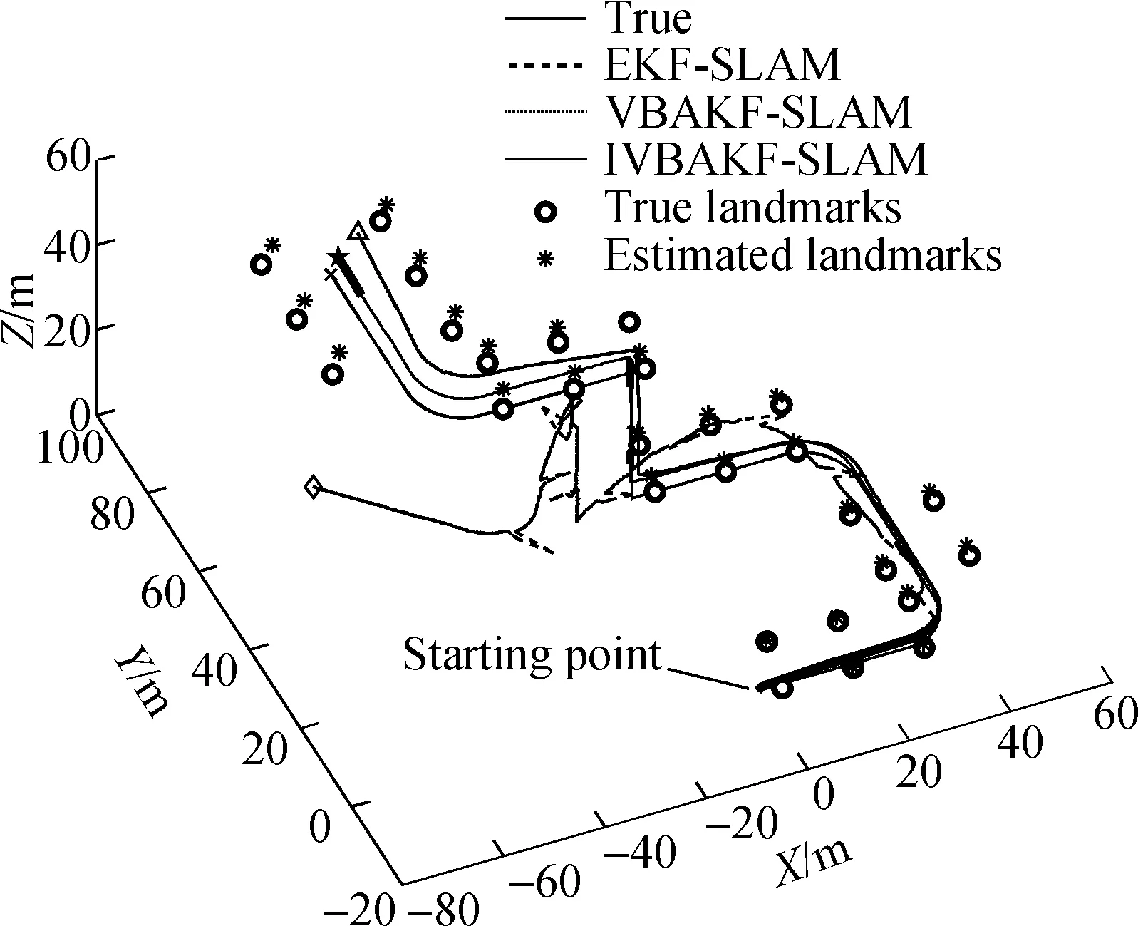
Fig.7 Estimation trajectory comparison in Experiment 3
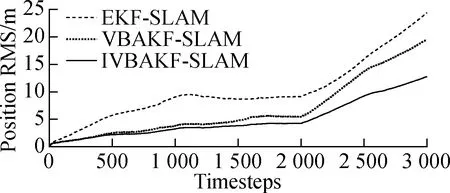
The pose estimation error and RMS value of the pose estimation error for the three algorithms are described inFigs. 8 and 9, respectively. In Fig. 8, the filtering effects of the three algorithms are the same in the timesteps of 0 to 500, and the fluctuation of the pose estimation error in thex,y, andzdirections and heading is very small. After 500 timesteps, the pose estimation error based on the EKF-SLAM method begins to increase gradually, and the maximum error value inydirection reaches 52.29 m. Meanwhile, the pose estimation errors based on the VBAKF-SLAM and IVBAKF-SLAM algorithms are relatively small, and the filtering effect of the IVBAKF-SLAM algorithm is optimal. Similarly, from the perspective of the RMS error of the position and heading angle, the RMS error of all three methods increases when the non-Gaussian noise and outliers appear in the measurement information. However, the RMS error curves of the EKF-SLAM method greatly fluctuate,and that based on the VBAKF-SLAM and IVBAKF-SLAM methods slowly increases.

(a)

(a)
Tab. 2 demonstrates the ARMS values of the vehicle estimation and features estimation observed for the three algorithms. In Tab. 2, the ARMS of the position estimation based on the IVBAKF-SLAM algorithm is 8.027 4 m, that of the heading estimation is 0.176 1 rad, and that of the feature estimation is 9.316 3 m. Therefore, compared with the other two methods, the filtering performance of the IVBAKF-SLAM algorithm is optimal.

Tab.2 ARMS for the three methods in Experiment 3
3 Conclusions
1) In practical applications, the statistical characteristics of the measurement noise are usually unknown and time-varying. It also has non-Gaussian distribution or outliers due to various factors, such as impulse noise or instantaneous interference.
2) All of these will result in the incorrect or even non-converged state estimation of the measurement update phase of the SLAM localization method. Based on this, a robust SLAM localization method based on the IVBAKF is proposed.
3) Three experiments are designed, and in the third set of the experiment, the positioning accuracy of the proposed method is improved by 17.23%, 20.46%, and 17.76% compared with that of the VBAKF-SLAM method. Therefore, the IVBAKF-SLAM method has better applicability and robustness to environmental interference.
 Journal of Southeast University(English Edition)2022年4期
- Journal of Southeast University(English Edition)的其它文章
- WinoNet: Reconfigurable look-up table-based Winograd accelerator for arbitrary precision convolutional neural network inference
- Damage identification of steel truss bridges based on deep belief network
- Deciding whether manufacturing firms share product links on owned social media considering fan effects
- Manufacturers’ channel selections under the influence of the platform with big data analytics
- Roughness evaluation of three-dimensional asphalt pavement based on two-dimensional power spectral density