
Analysis of anomalous transport based on radial fractional diffusion equation
2022-05-05 01:49KaibangWU吴凯邦LaiWEI魏来andZhengxiongWANG王正汹
Plasma Science and Technology 2022年4期
Kaibang WU (吴凯邦), Lai WEI (魏来)and Zhengxiong WANG (王正汹)
Key Laboratory of Materials Modification by Beams of the Ministry of Education, School of Physics,Dalian University of Technology, Dalian 116024, People’s Republic of China
Abstract Anomalous transport in magnetically confined plasmas is investigated by radial fractional transport equations.It is shown that for fractional transport models, hollow density profiles are formed and uphill transports can be observed regardless of whether the fractional diffusion coefficients(FDCs)are radially dependent or not.When a radially dependent FDCDα (r )<1is imposed,compared with the case underDα ( r)=1.0,it is observed that the position of the peak of the density profile is closer to the core.Further,it is found that when FDCs at the positions of source injections increase, the peak values of density profiles decrease.The non-local effect becomes significant as the order of fractional derivative α →1 and causes the uphill transport.However, as α →2, the fractional diffusion model returns to the standard model governed by Fick’s law.
Keywords: anomalous transport, hollow profile, non-locality, fractional diffusion equation
1.Introduction
Understanding the mechanism of transport is one of the most significant issues in magnetically confined plasmas.The standard transport model states that the transport fluxΓ is proportional to the local gradient of a physical quantityX,e.g., temperature, density, or energy, with additional convective termXV.Γ can be written in the mathematical form Γ = -D∇X+XV, whereDis the transport coefficient and Vis the convective velocity.Therefore,the transport equation has the form∂tX= -∇·Γ+S,whereSis a source.This implies that this model is based on a Markovian, Gaussian,uncorrelated process, because from the statistical point of view, if a system obeys the Gaussian distribution, the transport coefficient and convective velocity can be expressed asD=limt→∞σ2/tandV=limt→∞M/t,respectively, whereσ2is the variance andMis the mean.However, in magnetically confined plasmas, this model is insufficient to explain non-Markovian and non-Gaussian transport withσ2~tn,n≠1.For example,some experiments found non-local effect that when an edge cold pulse was imposed,the temperature at the core rose [1, 2].Some simulation results showed that the tracer particles are trapped in eddies or jump over several eddies in a single flight in a plasma with resistive pressuregradient-driven turbulence and the varianceσ2~tnwithn>1,which implies that the transport of tracer particles was super-diffusive and can be modeled by the fractional diffusion equation [3-5].In the plasma device TORPEX, suprathermal ions presented non-diffusive transport,forσ2~tnwithn>1 for super-diffusive orn<1 for sub-diffusive transport.The super-diffusive transport for suprathermal ions is related to large fluctuation, resulting in highly intermittent time traces,whereas the sub-diffusive transport does not present such intermittency [6, 7].Moreover, during off-axis electron cyclotron heating, the non-diffusive transport of temperature was observed in the DIII-D tokamak [8, 9], and hollow profiles of temperature were observed in the Rijnhuizen Tokamak Project[10].In the device HT-7 electron heat pinch was observed using off-axis ion cyclotron resonance frequency heating [11].Moreover, in Tore Supra, heat pinch effect was also observed and this effect was enhanced in low-density discharge [12].Further, hollow density profiles have been observed during the fueling processes in some devices[13, 14], and the related micro-turbulence studies have also been done [15-17], as well as the hollow profiles of impurities [18-20].Some simulations showed that tracer particles were trapped in eddies or jumped over several eddies in a single flight in a plasma with pressure-gradient-driven turbulence.
In recent years,fractional calculus has been applied to study non-local,non-diffusive transport.Mathematically,the fractional derivatives are defined through specific forms of integro-differential operators [21, 22] that generalize the definition of conventional differentiation.The numerical method is a significant topic as well [23] to study transport in complex systems.The one-dimensional fractional transport model has been proposed to study non-diffusive transport in magnetically confined plasmas[24].In fact,the fractional transport models are closely related to the continuous time random walk(CTRW)models,which allow a particle at positionxto have a jumpΔxafter a waiting time Δtdescribed by the probability distribution functions (PDFs)η(Δx)andψ(Δt)ifΔxandΔtare independent random variables [25].Moreover, a system without characteristic scale means that the second and higher moments of the underlying PDF do not exist, implying that heavy tail distribution (Lévy distribution)is allowed.Therefore, with the CTRW model, the generalized master equation can be derived [26].Due to the heavy tail distribution, it can be presented that uphill transport means that the flux flows along the direction of density gradient in a bounded domain [26-28].The radial fractional transport equation in polar coordinates can be derived from the CTRW model by azimuthally averaging the two-dimensional Laplacian operator[29,30].Moreover,the radial fractional diffusion model is consistent with experiment results in some devices [31].Another numerical method for two-dimensional fractional diffusion equations is the iteration method [32], which has been applied to model electron cyclotron resonance heating experiments in LHD [33].
The transport coefficients in general are not spatial-temporal invariant.Besides,the non-local effect plays a significant role in causing anomalous transport.Hence, the goal of this work is to investigate the effects of radially dependent FDCs on density profiles as well as the origin of non-locality through numerical methods.The paper is organized as follows:section 2 reviews the derivation details of the radial fractional transport model,section 3 compares the numerical results of density profiles under various fractional transport coefficients and source profiles,section 4 presents the origin of non-local effect via numerical study, and section 5 contains the summary and conclusions.
2.Radial fractional diffusion model
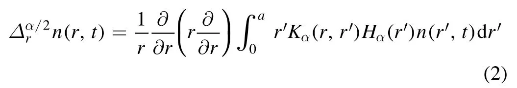
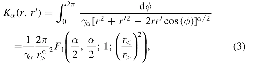
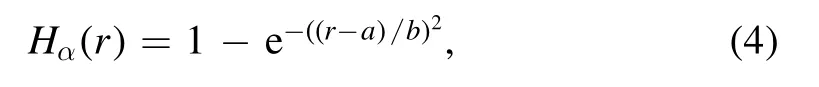
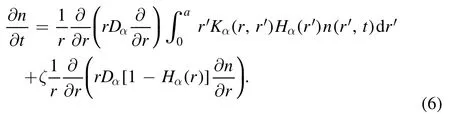
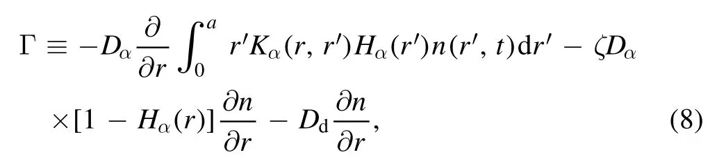
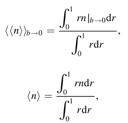
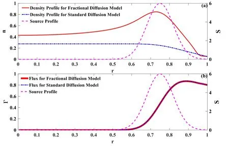
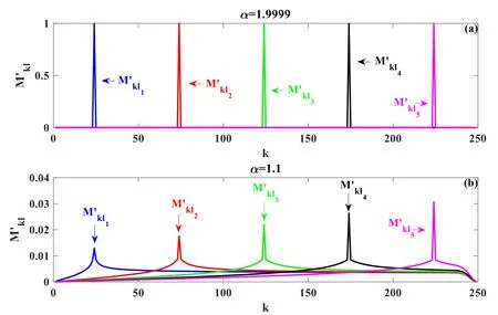
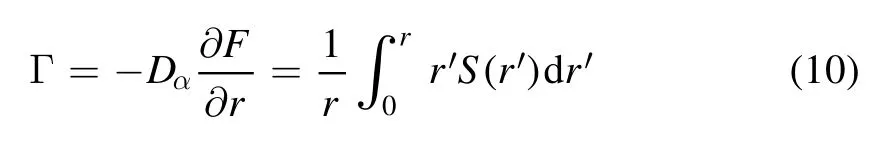
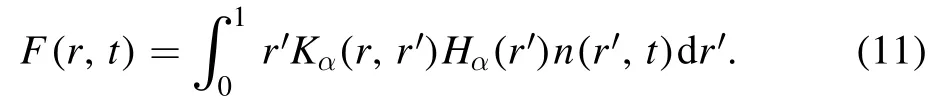
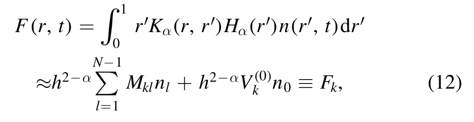
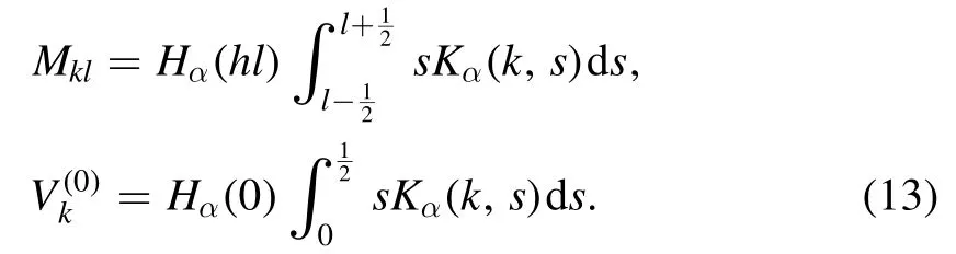
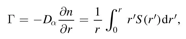
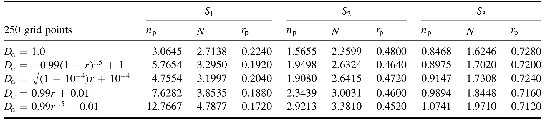
In[29-31],the radial fractional transport equation for densityn(r,t)with FDCDαin a bounded domain 0 where is the fractional Laplacian operator and the kernelK α(r,r′)is given by where2F1(i,j;k;z)is Gauss’s hypergeometric function[34]andr>=max {r,r′}as well asr<=min {r,r′}.Moreover,γα=π22-αΓ (1-α/ 2)/Γ(α/2).Note that the word‘fractional’denotesthat thefractional derivative isinvolvedinthe diffusion flux written as which is different from the standard diffusion flux-Dd∂n/∂r,whereDdis the standard diffusion coefficient.Parameterαis the order of the fractional derivative with interval1<α<2, implyingαis a fraction.The proportionality coefficientαDis the fractional diffusion coefficient.Whenα= 2,equation(1)returns to the standard radial diffusion equation based on Fick’s law.The purpose of the mask functionαH r( )is to guarantee that the integration on the right-hand side of equation (2)is finite if the boundary conditionsn(a)and∂rn(a)are nonzero.Therefore, the mask functionHα(r)can be written as subjected to the boundary conditions and the parameterbin equation (4)decides the width of boundary layer.WhenαH(r)is imposed, the densityn(r,t)away from the boundary layer is independent of the boundary conditions, sinceHα(r)anddHα(r)/drapproaches zero near the boundary layer.To satisfy the boundary conditions, we need an additional term for boundary layer with the form of conventional diffusion such that the fractional Laplacian operator is well-posed.Thus, when an FDC is radially dependent, the fractional diffusion equation has the form The first and the second terms on the right-hand side of equation (6)give the divergences of uphill and downhill transport fluxes, respectively.As mentioned in [29, 30], the uphill flux arises from non-local effect inside the boundary layer, and the downhill flux comes from the standard diffusion at the boundary layer.Moreover,when there is no source in the system, in a steady state the two fluxes should be balanced.Since the downhill flux is generated in the boundary layer,ζplays the role to decide its strength.Therefore, the parameterζdecides the strength of the boundary layer. Thus, when standard diffusion model and a source are taken into account, the diffusion equation reads and the particle flux is defined as whereSis a source.We further define the total number of particlesthe peak value of a density profilenp≡max(n), and its positionrp. In this section, equation (7)is solved numerically based on an explicit finite difference scheme.The dimensionless variables are defnied asr/a→r,b/a→b,t/t0→t,Dα t0/aα→Dα,Ddt0/a2→Dd,ζ/a2-α→ζ,whereais the minor radius,t0=a2/Dd0is the characteristic scale of the diffusion time(particle confinement time), andDd0=a2/t0is the characteristic diffusion coeffciient.For the source and density terms, the dimensionless variables are defnied asS/S0→Sandn/n0→n,wheren0=a2S0/Dd0is the characteristic diffusive scale of density andS0is the characteristic scale of the source term.In addition, the mask function can be written asHα(r)=1 -exp[ - (r-1)2/b2]. To investigate the influence of parameterbon density profiles in steady states, with the average density asb→0,the average density and the difference between them are calculated through andΔ〈n〉 = 〈n〉 - 〈n〉 ∣b→0,respectively.The source profile isS=Sscexp(-r2/0.22),whereSscis a constant such thatThe source is on-axis injected in order that we can investigate how the boundary layer itself could affect the density profiles in interior domain.As shown in figure 1,since〈n〉∣b→0approaches an asymptotic value due to∣Δ〈n〉 ∣→0regardless of value ofα,the relative error can be expressed as ∣Δ〈n〉 ∣/〈n〉∣b→0×100%.For example, ifα=1.1 andb=0.035, then the relative error ∣Δ〈n〉∣/nasym×100% ≈2.0% is obtained.Since there are few theoretical methods on how to decideαand the boundary layer widthb,the choice of values ofαandbin our work depends on experimental data.Therefore, to study the effect of nonlocality on density profiles and by referring to experimental data [13], we choose α = 1.1, b =0.025, which results in about 1.37% relative error. All of the numerical results are presented in the steady states,and therefore the initial condition ofn (r ,t)is arbitrary.The boundary conditions aren (r=1,t)=0.05and due to the symmetry of the system,∂ n /∂r∣r=0=0is set.The azimuthally symmetric (ring shape)source profile is assumed to have the form S =Snf (r ),whereSnis a constant such thatTo better model the experiment of off-axis fueling, the locations of source injections are away from the core.Figure 2 shows fractional and standard diffusions with red and blue curves, respectively.Note that the standard model applied in this section is Figure 1.Sensitivity of the average values of〈 n〉 to the parameter b.The calculation of the relative error is described in the text.In this figure,ζ = 1.0 is chosen. Figure 2.Profiles in steady states.Panel(a)shows the particle density and source profiles,and panel(b)illustrates the particle flux and source profiles.The blue and red curves correspond to standard and fractional diffusion models by ignoring Dα and Dd ,respectively.The magenta dashed curve is the source profile and One of the most significant features of radial fractional transport is the hollow density profile, as shown in figure 2 with the red curve.For fractional transport, the peak of the density profile is away from the origin and there exists a local minimum at the core whereas, for classical diffusion, there exists a local maximum at the origin of the density profile.Moreover, because∂ n /∂r > 0 for the red curve in the interval r< 0.72, and the fluxes are positive for both fractional and standard diffusions as shown in figures 2(a)and(b), the fractional transport exhibits uphill transport in this interval.However, for classical diffusion, the uphill transport does not exist because the flux always flows opposite to the density gradient.Besides,the total number of particles for the red curve is greater than that for the blue, which might be responsible for the fact that particles in the fractional transport diffuse slower than in the standard transport model. We next investigate the effect of radially dependent diffusion coefficients on density profiles.Generally speaking,the transport coefficient is not a constant in magnetically confined plasmas; it might depend on the topology of magnetic field, the collisional frequency, and so on.Some experiments showed that diffusion coefficients of particles increase from the core to the edge[35].From equation(7),the slope of an FDC would affect the density profile.Hence,four kinds of FDCs are assumed: concave down, concave up,linearly increasing, and constant.If FDCs are concave down,they increase faster near the core whereas, if FDCs are concave up, they increase slower near the core. The colored curves in figure 3 are profiles of FDCs, and their corresponding density and flux profiles are illustrated in figure 4.We ignore the last term on the right-hand side of equation (7)in order to investigate anomalous transport purely arisen from fractional transport.For source profiles,f (r )= e-(r-rn)2/0.12is set,where rn=0.25,0.50,and0.75 are positions of source injections forS1,S2,andS3, respectively.All of simulation results are summarized as in table 1.Note that in table 1,the total number of particlesthe peak value of a density profilenp≡max(n ),and its positionrpare defined. Figure 4 shows that the uphill transport exists,regardless of whether the FDCs are radially dependent or not.In the standard diffusion model, density profiles are peaked at the core.However, for fractional diffusion, the density profiles are peaked away from the origin.The positions of peaks of density profilesrps are around the source injection positions for fractional diffusion,as shown in figures 4(a)-(c),and they decrease if FDCs are radially monotonically increasing.Moreover,from table 1,it is found that the larger the FDC at the position of particle injection is, the smaller thenpis.Furthermore, for concave up profiles of FDCs, the total number of particles is larger than that for concave down ones. Figure 3.The fractional diffusion coeffciients applied in this work.The blue, magenta, green, red, and brown curves correspond to FDCs Dα=1.0,-0.99 (1-r)1.5+1,,0.99r+0.01, and0.99r1.5+0.01,respectively.The gray lines represent the positions of particle injections. Figure 4.The density,source,and particle fulx profiles in steady states for the diffusion coefficients shown in figure 2.For the source proflies presented by the gray curve,we assumewhere rn=0.25, 0.5, and 0.75for figures 4(a)-(c),respectively.Figure 4(d)shows particle fluxes in steady sates. Figure 5. andwhere andare grid points corresponding to r =0.1, 0.3, 0.5, 0.7, and 0.9, with blue, red, green, black, and magenta curves, respectively.When α →2, the values for each curve are zero except when k =l such thatwhereas for α →1, each curve has acertain value even if k ≠l, and that results in non-local effect. Figure 6.Areas AM under curves corresponding to each k of M ′kl. To compare with real experiment data, we setDd0=0.1 m2· s-1,S0=1019m-3·s-1,a=1 m,andn0=1020m-3,then density approximately reaches 5 ×10¹⁹m-3at the core and 1020m-3near the edge as shown in fgiure 4(c), which is consistent with experiment data after L-H transition as shown in figure 1(b)of[13] in order of magnitude. When a system is in steady state,from equations(7)and(8)in the interior of the domain, we obtain where From figure 4(d)and equation(10),the particle fluxes are positive, which means that particles flow outward.Besides,becauseis fixed, the maximum value ofΓ increases as the position of source injection approaches the origin. In the standard diffusion model,from Fick’s law,particle flux is proportional to the gradient of density, which can be expressed in mathematical form asΓd= -Dd∂n/∂r.In the fractional diffusion model, when the order of fractional derivativeα→2, the fractional diffusion model returns to the standard diffusion model [28].That is,F=asα→2, which impliesr′K α(r,r′)→δ(r-r′).In other words,r′Kα(r,r′)becomes localized and non-local effect is insignificant.This can be confirmed by numerical calculation.From [28, 29], if we divide [0, 1] withN+1 grid points, and grid sizeh≡ 1 /N, then equation (10)can be approximated as wheren0is the density at the origin,andk=1, 2,… ,N-1.We therefore have To investigate the effect of non-locality,we can fixlandα, and plotM′kl≡h2-αMklversus grid pointskas shown in figure 5.From figure 5(a),M′kl→δk-lasα→2,which meansF(r,t)→n(r,t)in equation (12).Thus,equation (10)can be written as which is equivalent to Fick’s model of diffusion. However,as shown in fgiure 5(b),M′klhas a certain value even ifk≠l.This is the origin of non-locality which should be taken into account when transport is analyzed.That is,F(r0,t)at a given pointr0is influenced by the values of density at other points,not justn(r0,t).From equation(12),Fkis related to the areaAMunder the curve ofM′klfor a givenk.Supposing that the observed density profile is a constant or concave down,the position of the peak of the corresponding particle flux will be near the boundary becauseAMdecreases askincreases as shown in figure 6,which is contradictory to the fact that particle flux peaks in interior domain.Thus, we conclude that the density profiles will be convex from the origin at first and reach maximum values at certain locations in steady states. From equation (10), we have whereΓeff≡Γ/Dαis effective flux.Compared with the location of the peak of the fluxΓ, if a monotonically increasing fractional diffusion coefficientDα(r)<1exists in the interior domain, from equation (14), the location of the peak of an effective flux is closer to the core under the same source profile.Thus, the positions of the peaks of density profiles also move to the core. In standard transport process, it can be described by the Brownian random walk model and the Gaussian probability distribution function is obtained.Therefore, the auto-correlation is exponential decay and the second moment is fniite.The former denotes short-range interactions;the latter shows that the system has a characteristic length, whereas, for a system with algebraically decaying distribution functiona significant feature is the existence of heavy tail distribution,and the Lévy flight random walk model is utilized to derive equations(1)-(3).Therefore,the auto-correlation is algebraically decaying and the second moment is infinite, which means that the displacements between two consecutive steps have correlation, and the system is scale free due to the absence of characteristic length.Moreover, because of heavy tail distribution,there is small probability for the occurrence of large fluctuations,which results in non-local effect. In this work,the fractional diffusion coefficients are assumed to be radially increasing functions from the core to the edge,which could model diffusion processes in real experiments.It is found that the hollow density profiles are formed regardless of whether the FDCs are radially dependent or not.Therefore, in some intervals, uphill transports can be observed.The peak values of density profiles are related to FDCs at the locations of source injections.That is, the smaller the FDC is at the position of particle injection,the greater thenpis.From figure 4 and table 1,as well as comparing with the position of the peak of density proflie withDα=1.0,we fnid that the positions of the peaks of density proflies are closer to the core under the same source proflie with radially dependent FDCsDα(r)<1.0.Moreover,a larger amount of particles can be obtained under a radially dependent FDC with a concave up proflie, which means the confniement time is longer and is beneficial for fusion reaction. Table 1.The total number of particles N, peak values of density profiles np, and their corresponding positionsrp are summarized. The non-local effect becomes significant if the order of fractional derivativesα→1.From the statistical point of view, an algebraically decaying distribution function possesses heavy tail distribution, which implies that large fluctuations exist to generate the non-local effect.For standard transport model (α→2), the Gaussian distribution function decays faster, such that small fluctuations dominate,demonstrating the absence of non-local effect. A continuous time random walk (CTRW)model was proposed in[25].This model is the generalization of the Brownian random walk model.In[26-28],the authors investigated particle transport through the CTRW model and observed uphill transports.Moreover,in[28],the fractional transport equations could be derived from the CTRW model in fluid limit.In[24,29-33],the authors applied fractional transport equations to model thermal transport and confirmed the existence of uphill transports.Note that in [30, 31], the authors utilized a radially fractional transport equation to model hollow temperature profiles as shown in figure 4 of [31].In our work, the factional transport equation is applied to model diffusion process, and the simulation results are consistent with real experiment data in order of magnitude.Thus,the fractional transport model can be applied in both particle and thermal transports. There are some experiments in which a cold pulse is suddenly launched at the edge of tokamak, and the temperature at the core simultaneously raises.Therefore, it strongly presents a non-local effect in thermal transport in plasmas.Since we focus on the formation of hollow density profiles and anomalous particle transport, anomalous thermal transport and mechanism of fast propagation of cold pulse will be explored in a future study. Acknowledgments The authors thank Dr Patrick Diamond for his comments on this work.This work is supported by the National MCF Energy R&D Program of China (No.2019YFE03090300),National Natural Science Foundation of China (No.11925501), and Fundamental Research Funds for the Central Universities (No.DUT21GJ204).


3.Numerical results


4.Effect of non-locality on density profiles

5.Conclusion
 Plasma Science and Technology2022年4期
- Plasma Science and Technology的其它文章
- Numerical analysis on the effect of process parameters on deposition geometry in wire arc additive manufacturing
- Investigation of the gas bubble dynamics induced by an electric arc in insulation oil
- The influence of charge characteristics of suspension droplets on the ion flow field in different temperatures and humidity
- Characteristic studies on positive and negative streamers of double-sided pulsed surface dielectric barrier discharge
- Hydrophobicity changes of polluted silicone rubber introduced by spatial and dose distribution of plasma jet
- Characteristics of water volatilization and oxides generation by using positive and negative corona