Approaches to quantify axonal morphology for the analysis of axonal degeneration

Alex Palumbo, Marietta Zille

Morphological hallmarks of axonal degeneration (AxD):

Axons transmit signals from one neuron to another and are crucial for the proper communication in the nervous system. Therefore, the disintegration of axons, a process named AxD, has detrimental consequences and plays a key role in many neurological diseases.

AxD is characterized by the formation of two morphological hallmarks, namely axonal fragments and axonal swellings. Whereas axonal fragments are separated segments of the axon resulting from axonal breakdown, axonal swellings are spherical structures that may emerge along the axon prior to the formation of axonal fragments (Palumbo et al., 2021). Quantifying these morphological hallmarks enables researchers to follow AxD over time, better understand differences in AxD kinetics, and assess candidate treatments.

Here, we give a brief overview of the different approaches to quantify AxD based on axonal morphology and explain how recent machine learning tools may be used to decipher the progression of AxD to further our understanding of this process and develop novel therapeutic interventions.

Image binarization and manual labeling to quantify AxD:

A widely applied approach to analyze AxD is the AxD index (or relative neurite/axonal integrity), the ratio of the fragmented axon area over the total axon area (Sasaki et al., 2009; Arrázola et al., 2019). To identify axons and axonal fragments, grey-scale microscopic images are converted to binary images by thresholding. Pixels are thereby assigned to background, axons or axonal fragments. Structures that are continuously connected are counted as axons, whereas axonal fragments are identified as non-connected structures and counted using the particle analyzer module of ImageJ. Further measures of AxD are: i) the distance between lesion site and axonal tip, ii) the distance between fragments, iii) the length of the axonal fragments, and iv) fragmentation rate. The above-described approaches can be applied

in vitro

,

ex vivo

, and also

in vivo

(Kerschensteiner et al., 2005; Knöferle et al., 2010; Gerdts et al., 2015; Canty et al., 2020). For the latter, fluorescently labeled axonal tracts using transgenic mice or viruses are required. However, image binarization is not always sensitive enough to recognize thin axons, which are then either omitted or misinterpreted as axonal fragments. Another drawback of image binarization is that it cannot be used to quantify axonal swellings.Approaches to investigate the occurrence of axonal swellings in

in vitro

,

ex vivo

, and

in vivo

experiments involve calculating i) the ratio of the number of axonal swellings compared to the axon length by manual labeling of regions of interest using ImageJ (Yong et al., 2019) and ii) the axonal swelling density measuring pixel intensity per axon length using MATLAB (Canty et al., 2020). As is the case for image binarization, these approaches are semi-automatic and subjective, because they require manual annotation, and thus are very time-consuming. Hence, a tool to analyze axonal morphology including both hallmarks of AxD – axonal swellings and axonal fragments – that is more objective and can be used automatically would be of great use to the scientific community.

Principle of deep learning to classify structures in microscopic images:

Recent progress in the field of machine learning has opened novel ways of how to quantify axonal morphology on microscopic images. Convolutional neural networks (CNNs) represent a deep learning approach to classify specific structures in microscopic images (Yang and Wang, 2020;

Figure 1

). A CNN consists of three different layers, namely input, hidden, and output layer, containing several nodes whose connection strengths are defined by weights.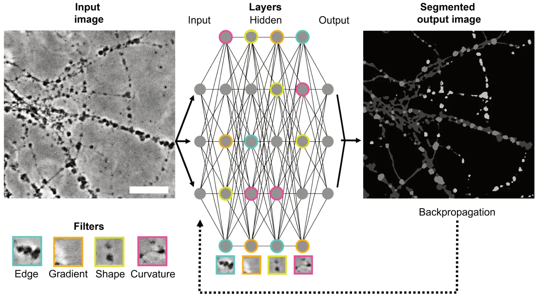

Figure 1｜Schematic illustration of the recognition of the morphology features of AxD by a CNN. A microscopic image containing axonal features (axons, axonal swellings, and axonal fragments) is introduced to the CNN as an input image. Each node of the input layer forwards dimensional pixel values to the hidden layers for structural information extraction via convolutional and pooling operations. In each of the hidden layers, nodes employ different filters (e.g., cyan filter for edges, orange filter for gradients, yellow filter for shapes, and purple filter for curvatures) and propagate the information to the nodes of the subsequent layer until reaching the output layer. In the output layer, all information is integrated to fully segment the input image. To correct potential errors in the output prediction of the CNN (dark grey = axons, light grey = axonal swellings, white = axonal fragments), backpropagation alters the connections among the nodes by readjusting the weights. Scale bar: 100 µm. AxD: Axonal degeneration; CNN: convolutional neural network. Unpublished data.

In the input layer, the CNN receives information about the dimensions of the images as input pixel values. The backbone of a CNN is the extraction of pixel information in the hidden layer by convolutional operations to recognize edges, lines, specific shapes, and gradient orientation. Convolutional operations are based on the application of different filters, also named kernels, that slide as a small window region over the image and calculate the sum of pixel values.To minimize the computational power necessary to process the data by reducing the image size, further pooling operations are employed for each area of the image covered by the kernel. During pooling, either the maximum or the average pixel value of the kernel covering an area of the image is extracted. Each pixel value originating from different kernels is then multiplied by an associated weight and transformed by a mathematical activation and normalization function to activate the node as it incorporates several weighted inputs. The activated node then propagates the information to several subsequent nodes in the next layer which differently weigh the input. These weight-associated node activations eventually determine which nodes are most strongly connected.

In the output layer, the probabilities of classifying specific structures in the microscopic image are calculated leading to the assignment of each pixel to a class (semantic image segmentation) as output. The resulting segmented image containing the classified pixels is then compared to the original image. A mathematical operation called “backpropagation” is eventually used to re-adjust the weights among the nodes in each layer to ensure that the output prediction of the CNN corresponds to the original image.

This learning process can be performed by the CNN itself or be taught via supervised learning (Yang and Wang, 2020). In the case of supervised learning, several microscopic images are annotated by experts. The original microscopic images and their annotations are “fed” into the CNN and used for output comparisons. Finally, the performance of a CNN to match the original image should be validated using independent datasets and compared against expert raters.

Deep learning-based approaches to quantify AxD:

Several CNNs have recently been developed for the recognition of axonal morphologies (

Box 1)

. TrailMap facilitates the 3D visualization of axonal projections in cleared brain tissue (Friedmann et al., 2020). The authors adapted the AdipoClear protocol to reduce the autofluorescence of myelin and axons of healthy brains that were fluorescently labeled by viral-genetic strategies. The recognized axons were then aligned to the different brain regions using the Allen Brain Atlas Common Coordinate Framework as a standard reference space. Using this approach, the authors were able to quantify axonal density within noisy whole-brain volumetric data. However, this tool is not suitable to determine AxD as it has not been trained to distinguish between healthy axons and axons undergoing AxD. In addition, although TrailMap identifies differently labeled axons originating from various neuron types, the resulting visualization does not discriminate between axons and dendrites.

Another tool developed by Schubert et al. (2019) allows to distinguish between neuronal substructures (axons, dendrites, and somata) using cellular morphology neural networks (CMN) based on multi-view projections. These networks combine unsupervised and supervised learning approaches to analyze electron microscopy images. In addition to the reconstruction of different neuronal substructures, the authors were also able to distinguish between various neuron types and glial cells. Despite the advantage of cellular morphology neural networks to reconstruct the axonal 3D shape from several multi-view 2D images, they have not been specifically developed to reconstruct fragmented axons.

AxonDeepSeg is another supervised CNN that can be used to segment axons and myelin in crosssectional electron microscopy images of brain and spinal cord tissue (Zaimi et al., 2018). The authors provide two ready-to-use models for scanning and transmission electron microscopy and demonstrated high segmentation accuracy across different species and tissues. Although this method allows to calculate the volume, diameter, and density of axons and myelin, which can be used as estimates to evaluate AxD, it does not consider axonal swellings as a direct morphological hallmark of AxD.

For axonal swelling recognition, Cheng et al. (2019) developed the DeepBouton supervised CNN. It counts the overall number of axonal swellings along individual neurons based on the different sizes and fluorescence intensities in confocal images of the whole brain of mice that the authors acquired by high-resolution stage-scanning microscopy. The method is superior to other conventional methods and can be used to detect axonal swellings in different neuron types.

Whereas whole brain or tissue section imaging is useful to determine AxD

ex vivo

at specific time points, it does not allow to examine the progression of AxD over time and to study the molecular machinery underlying AxD in its detail.

Cell culture systems allow to study spatially isolated axons by using a media volume difference that generates a microflux between a soma compartment and an axonal compartment. This microflux drives the outgrowth of axons from the soma compartment into the axonal compartment. Axons and somata can then be separately manipulated to assess different AxD stimuli. Recently, we have developed a microfluxbased cell culture system and the CNN-based deep learning tool EntireAxon to quantify axons, axonal fragments, and axonal swellings on microscopic phasecontrast images for AxD assessment (Palumbo et al., 2021). This allows the continuous detection of AxD over time without the need of expressing fluorescently labeled proteins or the fixation of the axons at different time points. The EntireAxon is trained to recognize the occurrence of axons, axonal swellings, and axonal fragments by segmenting each pixel of the image that is then classified as background, axon, axonal swelling, or axonal fragment. Further application of the EntireAxon on fluorescent images is also possible (Menon et al., 2020).

Based on the acquired data on the changes of morphological hallmarks of AxD over time, we were able to detect four morphological patterns of AxD (granular, retraction, swelling, and transport degeneration) in a model of AxD in hemorrhagic stroke (Palumbo et al., 2021). The EntireAxon tool cannot only assess AxD by quantifying the morphological hallmarks of AxD, but also determine the morphological heterogeneity of degenerating axons. This versatility may allow to expand our understanding of AxD in the context of neurological diseases. However, the EntireAxon CNN cannot be used to determine AxD on 3D images. Features such as branching, lengths, and diameters as well as tracking of axonal cargo transports are also of high relevance and subject of future development.

One of the main limitations of the currently available deep learning-based approaches is that they cannot quantify AxD

in vivo

. In the future, it is thus important to generate and share datasets to train CNNs that include

in vivo

microscopic recordings of axons undergoing AxD over time, which will enable the analysis of AxD progression in animal models. In addition, one of the general limitations in training neural networks is the availability of training data, which must be annotated manually by experts. To reduce labeling costs, active learning approaches can be applied to identify the images that yield the best results (Grüning et al., 2020), thereby saving time to implement or modify existing deep learning-based approaches.

Conclusions:

Recent deep learning-based approaches have significantly improved our abilities to quantify axonal morphological changes ensuring objectivity and automatization in the analysis process without the need for manual annotation and thresholding. This is of high importance to allow systematic investigation and to increase our understanding of the mechanisms underlying AxD. Together with enhanced throughput test systems, this will form a platform for the assessment of new drug candidates to prevent and treat AxD in many neurological diseases.

Box 1 Comparison of different deep learning-based approaches to quantify features of AxD:Deep learningbased approach EntireAxon (Menon et al., 2020; Palumbo et al., 2021) Specimen Whole tissue ex vivo TrailMap (Friedmann et al., 2020)CMN (Schubert et al., 2019)AxonDeepSeg (Zaimi et al., 2018)DeepBouton (Cheng et al., 2019)Whole tissue ex vivo Spatially isolated axons in microfluidic device in vitro Microscopy Light sheet microscopy Tissue slices ex vivoTissue slices ex vivo Phase-contrast and fluorescence microscopy, time-lapse imaging Networks 3D CNN based on u-net Electron microscopy Electron microscopy High-resolution stage-scanning confocal microscopy Cellular morphology neural networks based on multi view CNN CNN based on u-net CNN based on u-net with ResNet-50 Ensemble of CNNs, based on u-net with ResNet-50, recurrent neural network Learning strategy Supervised Supervised and unsupervised Supervised Supervised Supervised Recognized structures Axonal swellings Axons, axonal swellings, and axonal fragments Outcome parameters Axons Axons, dendrites, and somata Axons and myelin Axon density Reconstruction of volume and localization of axons, dendrites, and somata Volume, diameter, and density of axons and myelin, G-ratio Number of axonal swellings Area of axons, axonal swellings, and axonal fragments, degeneration patterns

This work was funded by the Fraunhofer Society, grant number 600199, and by Joachim Herz Stiftung, grant number 850022 to MZ.

Alex Palumbo, Marietta Zille

Department of Neurobiology, Harvard Medical School; Department of Cancer Biology, Dana-Farber Cancer Institute, Boston, MA, USA (Palumbo A)

Department of Pharmaceutical Sciences, Division of Pharmacology and Toxicology, University of Vienna, Vienna, Austria (Zille M)

Correspondence to:

Marietta Zille, PhD, marietta.zille@univie.ac.at.

https://orcid.org/0000-0002-0609-8956 (Marietta Zille)

Date of submission:

January 5, 2022

Date of decision:

February 7, 2022

Date of acceptance:

February 17, 2022

Date of web publication:

July 1, 2022

https://doi.org/10.4103/1673-5374.34390

4

How to cite this article:

Palumbo A, Zille M (2023) Approaches to quantify axonal morphology for the analysis of axonal degeneration. Neural Regen Res 18(2):309-310.

Open access statement:

This is an open access journal, and articles are distributed under the terms of the Creative Commons AttributionNonCommercial-ShareAlike 4.0 License, which allows others to remix, tweak, and build upon the work non-commercially, as long as appropriate credit is given and the new creations are licensed under the identical terms.