Modeling of beam ions loss and slowing down with Coulomb collisions in EAST

Yifeng Zheng(郑艺峰)， Jianyuan Xiao(肖建元)，†， Baolong Hao(郝保龙)， Liqing Xu(徐立清)，Yanpeng Wang(王彦鹏)， Jiangshan Zheng(郑江山)， and Ge Zhuang(庄革)

1School of Nuclear Science and Technology，University of Science and Technology of China，Hefei 230026，China

2Key Laboratory of Optoelectronic Devices and Systems，College of Physics and Optoelectronic Engineering，Shenzhen University，Shenzhen 518060，China

3Institute of Plasma Physics，Chinese Academy of Sciences，Hefei 230031，China

Keywords: NBI fast ion loss，slowing down process，EAST，Coulomb collisions

1. Introduction

In tokamak devices，the fusion reaction，neutral beam injection(NBI)，and radiofrequency heating will produce many energetic ions.[1]The energetic ions have sufficient strength and locality to cause damage to the surface of the device.[2]Compared with other auxiliary heating methods，NBI heating has the advantages of simple physical mechanism， high heating efficiency，and less coupling problems with the plasma.[1]In addition，NBI is also a current driven method.[3]Therefore，it has become a widely used auxiliary heating method in various experimental devices and has good heating effect. In practice， it is expected that the beam energy will be deposited as close to the plasma core as possible to heat the core plasma.The incident neutral beam particles are ionized into fast ions through charge exchange and collisions with the background plasma. The fast ions then transfer energy to the background electrons and ions through Coulomb collisions. The confinement，deposition，and diffusion of NBI fast ions are important topics in plasma theory and experiment.[4，5]In these topics，Coulomb collisions play a key role because it leads not only to the exchange of momentum and energy between the fast ions and the background plasma，but also to the redistribution of the fast ions.[6]Theoretically，the process of Coulomb collisions can be solved by the Fokker–Planck (FP) equation.[6]Since the densitynof NBI fast ions is much lower than the densitynbof the background plasma，i.e.，n ≪nb，we can consider the fast ions as test particles that are slowed down and deflected by multi-body Coulomb collisions with the background plasma.[4，5]

In addition to Coulomb collisions， fast ion loss is another factor that can affect the efficiency of energy deposition.Under the influence of magnetic field gradient and curvature，some NBI fast ions will experience prompt loss because of magnetic gradient and curvature drift and move out of the LCFS or hit the FW. The prompt loss not only reduces the plasma heating efficiency and energy confinement time， but also causes serious damage to the FW.[7]Besides，the prompt loss of fast ions has a non-negligible effect on the radial electric field and the poloidal electric field rotation changes of the edge plasma.[5，8–10]In addition to prompt loss， the pitch angle scattering loss and stochastic diffusion loss caused by Coulomb collisions are factors that will lead to the continued loss of fast ions. There are many other mechanisms for fast ion loss， which can be classified into two types. One is the loss caused by asymmetric magnetic field such as the ripple field，[11–13]the error field generated by the test blanket module，[14]and the field generated by the resonant magnetic perturbation coils.[15，16]The other is the loss caused by the three-dimensional (3D) disturbances such as the Alfv´en modes， sawtooth， and neoclassical tearing modes driven by fast ions.[17，18]In this paper，only the prompt loss and fast ion loss caused by Coulomb collisions are considered. In contrast to the calculation of the slowing down process which requires the evolution of the distribution function， the calculation of the fast ion loss requires the trajectory of each particle. Since the FP equation is a function of the distribution function， it may not accurately describe the trajectories and losses of individual particles. In order to obtain the information of distribution function evolution and single-particle trajectory simultaneously， we can convert the calculation of distribution function evolution into the calculation of single-particle trajectory directly based on the stochastic equivalence between FP equation and Stratonovich SDE.[19–21]Then， the distribution function can be obtained from the statistics of the particle trajectories. The macroscopic physical quantities are obtained by integrating the corresponding microscopic physical quantities over the distribution function.With the construction of high-performance computing clusters， the particle-based models can gradually handle multiscale and multi-degree-offreedom plasma physics simulations with Coulomb collisions.

Many orbit-following codes， such as ORBIT，[22]GYCAVA，[15，23]OFMC，[24]ASCOT，[25]SPIRAL，[26]and VENUS-LEVIS，[27]have been developed to study loss and transport of fast ions. These codes solve the guiding-center orbit or full orbit of particles， or both of them， such as ASCOT， SOFT， and VENUS-LEVIS. For guiding-center orbit programs，such as ORBIT，GYCAVA，only the guiding-center motion of the particles needs to be considered， thus saving computational costs. Moreover， the guiding-center orbit programs based on magnetic surface coordinates can provide a better physical interpretation. For full-orbit-following programs， such as SOFT and SPIRAL，the particle losses on the first wall of the tokamak can be calculated，while the magnetic surface based guiding-center orbit programs can only calculate the losses on the LCFS.In addition，for large variations in magnetic field gradients within a gyro-orbit，such as complex perturbation fields， the results of full-orbit-following calculations are more accurate.As a full-orbit following program，the Monte Carlo parallel program ISSDE uses the splitting method to construct the volume-preserving algorithms (VPAs)[28–30]for the collisionless part like the SOFT program. Based on this，ISSDE treats the collision part as a subsystem divided by the splitting method and uses an implicit midpoint format to enhance the long-term stability of the collision part.The simulation results compared with the analytical solution have been presented in Ref. [19]. The long-term stability of the algorithm is beneficial for the multiscale properties of fast ion loss and slowing down. On the one hand，as the fast ions carry energy，the simulation of short timescale fast ion loss will affect the long timescale fast ion slowing down. On the other hand，Coulomb collisions will induce the pitch angle scattering loss for marginal fast ion in a short timescale and the stochastic diffusion loss for fast ion near the plasma core in a long timescale. To calculate the fast ion loss and slowing down in EAST， we set up interfaces in ISSDE for the device and physical parameters， including the equilibrium configuration provided by EFIT，the initial distribution of fast ions provided by NUBEAM (a module extracted from TRANSP)，[31]and the temperature and density profiles of the background plasma that can be used to calculate the collision coefficients.

The rest of paper is organized as follows.In Section 2，the basic algorithm of the ISSDE program，the background plasma equilibrium configuration in tokamaks， and the initial distribution of NBI fast ions are presented. Combining information on fast ions in position space andPζ–Λspace， we present in Section 3 the prompt loss and orbit types of fast ions when the boundaries are LCFS and FW; pitch angle scattering and stochastic diffusion due to short and long timescale collisions;and slowing down process of fast ions. In Section 4，we summarize the main results.

2. Implicit Monte–Carlo full-orbit-following parallel program ISSDE and simulation parameter settings

ISSDE[19]is a Monte–Carlo full-orbit-following parallel program based on the implicit midpoint format of Stratonovich SDE，the splitting method and the quasi-Newton method.[20，21]In calculating the fast ion loss in EAST，the interfaces of EFIT and NUBEAM have been set up in the program to set the equilibrium configuration parameters and the initial distribution of fast ions. In the simulation， EFIT is used to get the equilibrium configuration of EAST，and NUBEAM is used to calculate the initial distribution of NBI fast ions，[31]and then bring the plasma parameters of the equilibrium configuration and the initial distribution of fast ions into ISSDE as input parameters.ISSDE can track the trajectory of fast ions and get the ensemble average physical quantities of slowing down process.

2.1. Numerical discrete method and new development of ISSDE

The algorithm of ISSDE is an implicit midpoint collision algorithm based on Stratonovich SDE. Its basic principle is the equivalence relationship between FP equation and Stratonovich SDE.Here，we give the basic equations required for the discretization of the algorithm; more details， such as the definition of each symbol in the equations， can be found in Ref.[19]. When calculating the NBI auxiliary heating，we assume that the background plasma is in equilibrium. When the background plasma reaches equilibrium， the corresponding distribution is the Maxwellian distribution，i.e.

In contrast to the study of uniform beam slowing down in static uniform fields in the Ref.[19]，in this work the curvature and gradient effects in the actual tokamak toroidal field are considered and the static field can be replaced by a quasi-static field as needed. We also changed the ion source from a simple uniform-beam ion source to an NBI fast ion source that conforms to the distribution of the neutral beam ionization law.The benchmark of the particle orbit is shown in Fig. 1. The full orbit calculated by ISSDE without collision is in consist with the guiding-center orbit calculated by the guiding-center algorithm provided by PTC code.[32]The PTC code has been compared with the ORBIT code. The benchmark of Coulomb collisions part with the analysis solution has been given in Ref.[19].

2.2. The equilibrium configuration and the initial distribution of fast ions

In our simulation，we use EFIT to obtain the equilibrium configuration[33]of EAST at the initial moment.In cylindrical coordinates，the relationship between the EAST magnetic field strengthBexpression and the poloidal magnetic fluxψis

whereψis the poloidal magnetic flux function， andg(ψ) is the poloidal current function. For a givenψandg(ψ)，we can calculate the value of each component of the magnetic field through Eq. (11). EAST is an all-superconducting tokamak.The first discharge was successful in 2006. The main parameters of EAST are as follows: the large radius is 1.75 m， the small radius is 0.4 m， the elongation is 1.6–2， the triangularity is 0.5–0.7， and the practical performance parameter of the toroidal magnetic field strength is 1.6 T–2.3 T. The typical physical parameters are: the average electron density is 1×1019m-3–5×1019m-3，the center electron and ion temperatures are 2 keV–4 keV and 1 keV–2 keV，respectively.[1，34]Enter the device parameters and the measured plasma parameters into EFIT to reconstruct the equilibrium. EFIT reconstructs the two-dimensional tokamak equilibrium by solving the Grad–Shafranov(GS)equation while maintaining the experimental measurements approximately. Equilibrium reconstruction can provide information on plasma shape and energy storage needed for plasma operation and experimental data interpretation， and can provide the magnetic field， current and pressure distribution needed for transport and stability researches.[33，35]

According to EFIT， we get the poloidal magnetic flux at 4.5 s for EAST discharge #93910 as shown in Fig. 2(a).The corresponding magnetic field configuration is the double null position type， the position of the magnetic axis is(1.9721，0.043)m，the solid red line represents the LCFS，and the black solid line represents the FW.Using the Eq.(11)we can calculate the corresponding magnetic field intensity distribution as shown in Fig. 2. The toroidal magnetic fieldBφdecreases continuously along the major radius as shown in Fig. 2(b). The poloidal magnetic fieldBθis distributed as shown in Fig. 2(c). Within the LCFS， the poloidal magnetic field rotates clockwise. Due to the gradient and curvature of the magnetic field， the fast ions have gradient and curvature drift motions that produce motion across the magnetic field lines. Through coordinate transformation， we can obtain the expression of magnetic field strengthBin the Cartesian coordinate system as

According to the Eq.(12)，we can calculate the magnetic field strength at any point in tokamak in the Cartesian coordinate system and then put it into the Eq.(10)to calculate the particle trajectory.

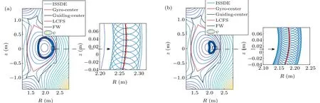
Fig.1. Comparison of the full-orbit calculated by ISSDE and guiding-center orbit calculated by the algorithm provided by PTC without Coulomb collisions.

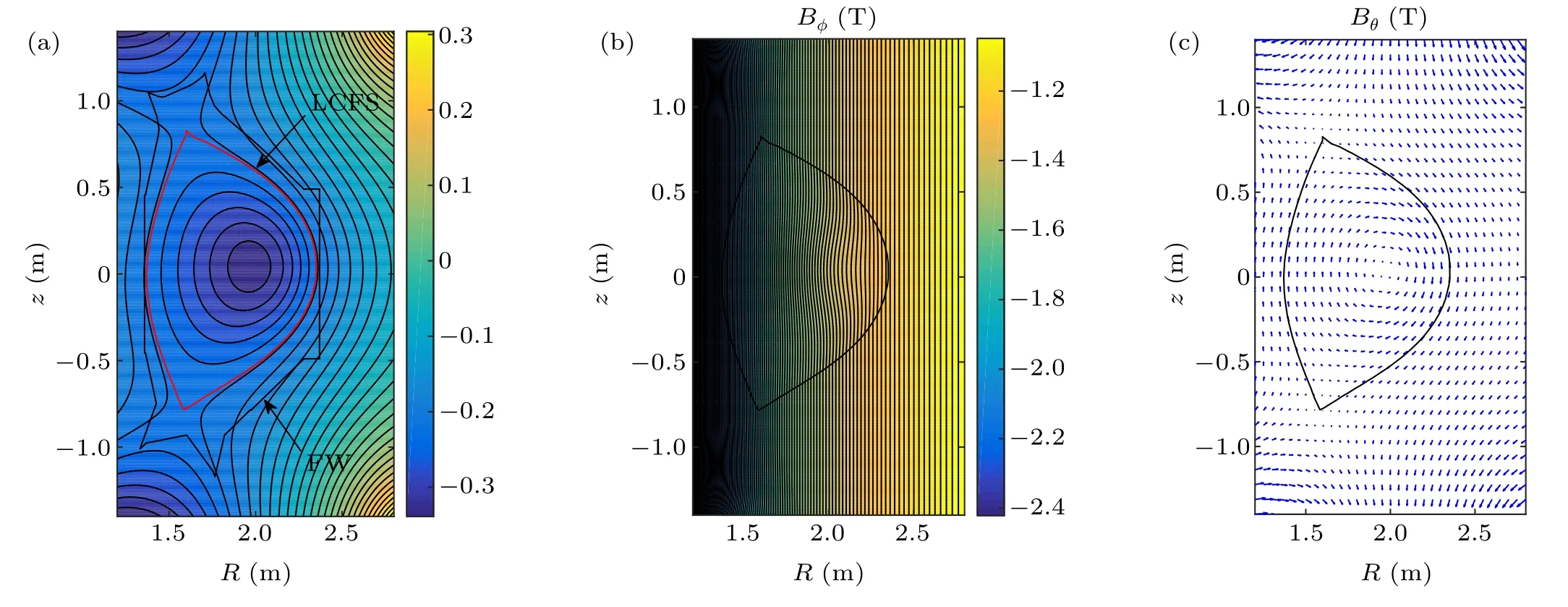
Fig.2. Poloidal magnetic flux and magnetic field intensity components Bφ and Bθ for EAST discharge#93910 at t=4.52 s.

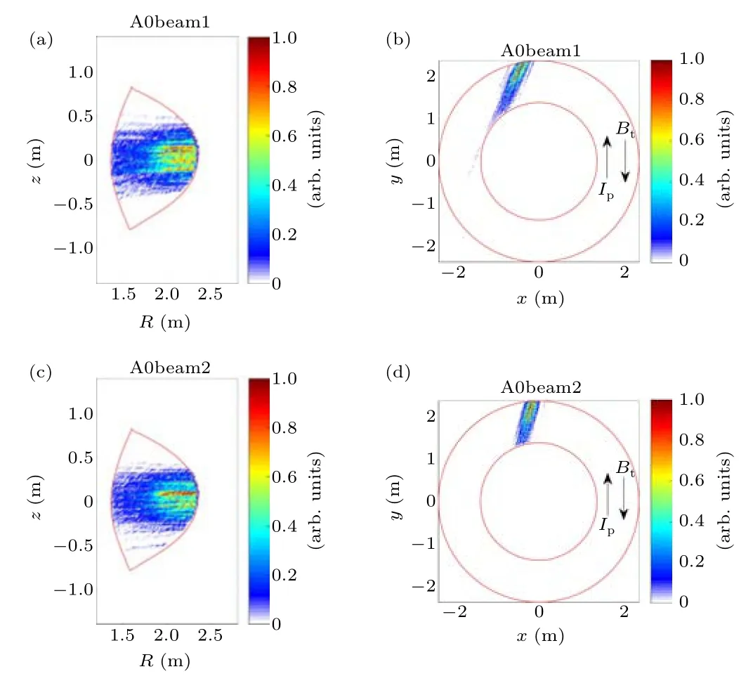
Fig. 3. The initial position distribution of fast ions obtained by NUBEAM:(a)and(b)for the tangential injection beam，(c)and(d)for the perpendicular injection beam.

Fig.4. Parallel velocity distribution of fast ions obtained by NUBEAM:(a)for the tangential injection beam and(b)for the perpendicular injection beam.

Fi g. 5. Pitch angle distribution of fast ion fromNUBEAM: (a) for the tangential injection beam and(b)for the perpendicular injection beam.

After the neutral beam is injected into the plasma， it generates fast ions through collision ionization process. The NBI system on EAST uses two deuterium beamlines with a power of 2 MW–4 MW and a beam energy of 50 keV–80 keV. NUBEAM is a widely used Monte–Carlo package for Tokamak fast ion deposition evolution，slowing down，and heating.[1]NUBEAM can calculate both the distribution function of fast ions by neutral beam deposition and by the fusion reaction.[36]Using NUBEAM，we can get the initial distribution of fast ions as shown in Figs.3–5. The tangency radii of the two beamlines corresponding to window A are 1.264 m and 0.731 m. Figures 3(a)and 3(c)are the initial position projections of the fast ion on the poloidal plane of tangential and perpendicular injection beams， and figures 3(b) and 3(d) are top view of the initial position of the fast ion of tangential and perpendicular injection beams. Where A0beam1 is the tangential injection beam，and A0beam2 is the perpendicular injection beam. The red line represents the LCFS.We see many lines in the NUBEAM results because，in the NUBEAM module， each beamline is represented by a probability-weighted randomly chosen collection of neutral tracks characterized by parameters that are input to the NUBEAM module.And a random choice of the deposition point is taken from a perturbed probability distribution to generate the initial condition for a Monte Carlo ion from a sample beam neutral trajectory.[37，38]The neutral injection beam contains a particle fraction with a total energy ofE1， a particle fraction with an energy ofE2=1/2E1， and a particle fraction with an energy ofE3=1/3E1. At the initial moment， the total energy of the tangential injection beam isE1=65.224 keV， and the proportions of each fraction are 69.54%， 23.14%， and 7.32%. The total energy of the perpendicular injection beam at the initial moment isE1=65.644 keV，and the proportions of each fraction are 65.55%， 12.58%， and 21.87%， respectively. It shows the parallel velocity distribution of fast ions in the major radius direction in Fig. 4. And it shows the pitch angle distribution of fast ions at the initial moment in Fig. 5. For the perpendicular injection，the fraction of particles whose pitch angle is close to 90°is larger. Therefore，for the case of perpendicular injection，the fraction of banana fast ions is larger.

Fig. 6. Electron density and temperature distribution profile for EAST discharge#93910.

2.3. Handling of Coulomb collisions in ISSDE

After obtaining the EAST equilibrium configuration and the initial position and velocity distribution of the fast ions，we can calculate the trajectory of each fast ion by ISSDE.Because the collision coefficients are functions of the background particle density and temperature，it is necessary to get the background density and temperature value at the local position of the fast ions and then bring it into the solution for the corresponding collision coefficients. It shows the background electron density and temperature profile in Fig.6. We assume that the background ion temperature and density have the same profile as the background electron. We can obtain the background density and temperature at the local position of the fast ion with the interpolation method. For the background plasma temperature and density outside the LCFS，we use the values corresponding to the LCFS in the simulation.

3. Fast ion loss and slowing down

NBI fast ions transfer energy to the background plasma through momentum exchange and energy exchange. Because of the bending and inhomogeneity of the magnetic field， fast ions will undergo curvature drift and gradient drift and move across the magnetic field lines. Some fast ions will eventually hit the FW and be lost. Using the Monte–Carlo full-orbitfollowing parallel program ISSDE and combining the information of fast ions in the position space and thePζ–Λspace，we can calculate the prompt loss and orbit types of fast ions when the boundaries are LCFS and FW.The pitch angle scattering loss，stochastic diffusion loss and the slowing down process under the effect of Coulomb collisions will be presented.

3.1. The prompt loss of fast ions with LCFS boundary and FW boundary

We calculate the prompt loss of fast ions with LCFS boundary and FW boundary.[39]According to the settings of the equilibrium parameters and the initial position and velocity distribution of fast ions，we use ISSDE to calculate the trajectory of fast ions and get the ensemble behavior by the statistic method. Numerical parameters are shown in Table 1， whereTic=4.07385×10-8s is the cyclotron period of the fast ion when the magnetic field strength is-1.61 T.

Table 1. The numerical experiment parameters of fast ion loss in EAST.

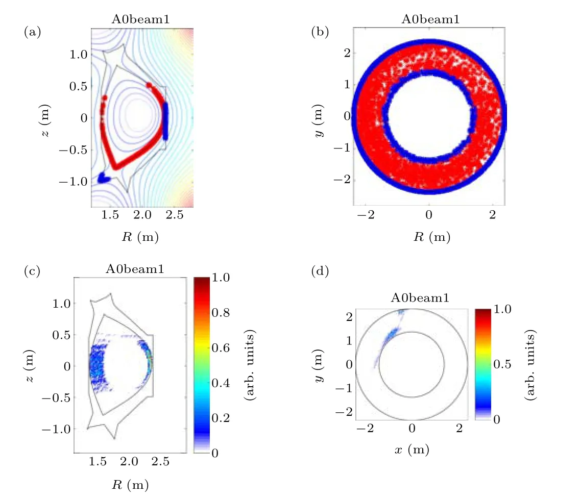
Fig.7. The fast ion loss position of the tangential injection beam，panels(a)and(b)are the positions of the lost particles at the time of loss，panels(c)and(d)are the positions of the initial time of the lost particles，red indicates that the loss boundary is LCFS， and blue indicates that the loss boundary is the FW.

Fig. 8. The fast ion loss position of the perpendicular injection beam， panels(a)and(b)are the positions of the lost particles at the time of loss， panels (c) and (d) are the positions of the initial time of the lost particles， red indicates that the loss boundary is LCFS， and blue indicates that the loss boundary is the FW.

We obtained the distribution of the lost positions of the fast ions at the final and initial moments， as shown in Figs.7 and 8.The positions of the loss particles are all below the midplane，which is related to the direction of the toroidal magnetic field. When the toroidal magnetic field is clockwise，the direction of the toroidal magnetic field gradient points to the center of the torus，so the force direction of the fast ions on the weak magnetic field side is from the strong magnetic field side to the weak magnetic field side， so the corresponding gradient drift is downward. The direction of curvature is outward along the major radial direction， so the centrifugal force on the fast ions is outward. Thus， the corresponding direction of curvature drift is also downward. Therefore，the lost position of fast ions will be below the mid-plane. The initial positions of lost ions are on the weak field side. The red points are the loss position of the ions when the loss boundary is LCFS，and the blue points are the loss position of the ions when the loss boundary is FW. It can be seen from panels (a) and (b) of Figs. 7 and 8 that the lost position of the fast ions in the FW is near the mid-plane and near the divertor. Because of the large gyration radius of fast ions，some ions that have drifted out of the LCFS will drift back into the LCFS and be captured again by the magnetic field. The comparison graphs(Figs.7 and 8(a))show that the lost position of fast ions for the perpendicular injection beam includes the high field side divertor，midplane，and the low field side midplane. While the lost position for the tangential injection beam includes the high field side divertor and the low field side mid-plane. We can see from panels(c)–(d) that for the co-current injection beam， the initial position of the lost fast ions is near the high field side. These results corroborate the findings of a great deal of the previous work in Xuet al.[16]

It shows the ratio of fast ion loss with and without Coulomb collision in the Table 2. Since the current is counterclockwise，A0beam1 and A0beam2 are both co-current beams.We can see that more fast ions of the perpendicular injection beam will be lost than the tangential injection beam. When Coulomb collisions are taken into account，the loss of particles increases. Comparing the prompt loss of the fast ions with the LCFS boundary and FW boundary，for the tangential injection beam，4.52%of the ions will not be lost after drifting out of the LCFS.For the perpendicular injection beam，this ratio reaches 5.11%. Therefore，the fraction of lost particles calculated with the FW boundary is more instructive for the actual physics of the perpendicular injection beam. At 8000Tic， the total loss in the perpendicular injection is greater than the loss in the tangential injection， and the time evolution of prompt loss is shown in Fig.9. In addition to the data information related to the loss fraction given in Table 2， in Figs. 9(a) and 9(b)， we can also get the information about the fast ion loss rate as follows. Firstly， in the first 1000Tic， the loss rate of fast ions is significantly higher than the average level because almost all particles can complete a bounce period in the first 1000Tic.Without Coulomb collisions or wave field disturbance， rest particles can be well confined， as seen from Fig. 9(a). Secondly，the loss rate of the LCFS boundary condition is greater than that of the FW one because the loss of particles in SOL also takes a certain amount of time.

Table 2.Fast ion loss ratio with and without Coulomb collisions at 8000 Tic.

Fig. 9. The evolution of fast ion loss with the LCFS and FW boundary for tangential and perpendicular injection: (a)for collisionless case，(b)for collision case. The solid lines represent the tangential injection beam， and the dashed lines represent the perpendicular injection beam. The blue lines represent the FW boundary and the red lines represent the LCFS boundary.

The loss rate of fast ions for perpendicular injection is greater than that for tangential injection，which is related to the orbital types of fast ions and the fraction of particles of these different orbital types. It can be seen from Figs. 10–13. Besides the spatial information of fast ions，the distribution of fast ions inPζ–Λspace is a necessary perspective to understand the type of particle orbits. Here，Pζis the regular momentum of the particle，Λ=μB0/E，μ， andEare the magnetic moment and energy of the particle， andB0is the magnetic strength at the magnetic axis. These parameters can be defined using the following formula in the full-orbit simulation，

Herevis the particle velocity，v‖andv⊥are the parallel and perpendicular components of the particle velocity，ψp，Bare the poloidal magnetic flux and the magnetic field strength at the particle location. Through the initial distribution of fast ions at thePζ–Λspace， we can get more information about the particle orbital type，[22]as shown in Fig.10. For the case of fixed energy， according to thePζ–Λvalue of the particle on the magnetic axis(dotted line)， thePζ–Λspace is divided into regions of different particle orbital types as following:(i)the maximum magnetic field intensity of the LCFS(black long dashed line)， (ii) the minimum magnetic field intensity of the LCFS (solid black line)， (iii) the capture-passing orbit boundary (based on the condition ofv⊥=0， black short dashed line)， (iv) and the maximumPζvalue under fixedμvalue (the upper black solid line). From Fig. 10， we can see that the fraction of passing ions is larger than that of the banana ions for both tangential beam and perpendicular injection beam. The proportion of trapped confined ions in the perpendicular beam is larger than that in the tangential beam. The proportion of co-passing confined ions in the perpendicular beam is smaller than that in the tangential beam. Co-passing orbit is the main orbital type for lost ions in tangential and perpendicular beams. Moreover，the proportion of banana lost ions in the perpendicular beam is larger than that in the tangential beam. By tracking the particles to 8000Ticwith ISSDE，we get the distribution of all lost particles with energiesE1，E2， andE3in thePζ–Λspace at the initial moment as shown in Fig. 11. The actual particle loss position is the same as the area marked in thePζ–Λspace，which verifies the correctness of the calculation. We use blue， and red circles to mark the location of the loss caused by Coulomb collisions in thePζ–Λspace. For tangential beams， the proportion of passing particles in this part of particles is higher， while for perpendicular beams， the proportion of trapped particles in this part is higher. The loss positions and fraction of different orbital particles in the position space are shown in Figs. 12 and 13.Here， the blue “+” represents the lost banana particles， while the red“*”represents the lost passing particles. The gray areas P1， P2， P3， and P4 are the lost regions. The passing ions in the tangential beam and the perpendicular beam are lost at the divertor position on the high field side and the midplane on the low field side， while the trapped ions are lost at the midplane on the low field side. Att=900Tic， for the tangential beam，the main loss particles are the passing particles and the loss ratio at P4 accounts for 84.52%of the total loss. For the perpendicular beam， 0.37% of the passing particle loss is at the mid-plane of the high field side，namely at P1，and the loss ratio of trapped particles is 20.58%， which is higher than the loss ratio of trapped particles in the tangential beam.

Fig.10. The Pζ–Λ space distributions of the beam ions in Fig.3 for different energy components: (a)E1，(b)E2，and(c)E3. Here，Λ =mB0/E with B0 is the magnetic strength at the magnetic axis，E is the particle energy，the toroidal momentum Pζ is normalized by qψw，and ψw is the poloidal flux at LCFS.The solid black lines show the boundary on the high field side of the LCFS corresponding to the fixed energies.While the black long dash lines show the boundary on the low field side of the LCFS.Particles have different orbit types in different regions in Pζ–Λ space，P-–L represents the counter passing-lost region，P-–C represents the counter passing-confinement region， P+–L represents the co-passing-lost region， and P+–C represents the co-passing-confinement region.The blue and red dots correspond to the tangential beam and perpendicular beam ions in Fig.3.

Fig.11. The distribution of all lost ions and the lost ions caused by collisions in the Pζ–Λ space at the initial moments. The red and blue dots indicate the initial positions of all lost ions of the tangential beam and the perpendicular beam，and the red and blue circles indicate the initial positions of the lost ions caused by Coulomb collisions of the tangential beam and the perpendicular beam.

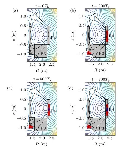
Fig.12. The fraction of lost passing and banana particles at position within the gray areas P1， P2， P3， and P4 at different time in the case of tangential injection. The red“*”represents the lost passing particles and the blue“+”represents the lost banana particles. At 900 Tic， the fraction of lost passing particles at P1，P2，P3，and P4 is 0%，14.25%，0%，and 84.52%respectively，while the fraction of lost banana particles at P1， P2， P3， and P4 is 0%， 0%，0%，and 1.22%respectively.

3.2. Fast ion loss caused by Coulomb collision

From the above analysis， we can see the prompt loss of fast ions and the type of fast ion orbits from the initial distribution of fast ions in thePζ–Λspace. To explore the effect of Coulomb collisions on fast ion losses and orbit types，fast ions that change their parallel velocity sign will be labeled as banana particles， and ISSDE is used to track the particle’s orbit and calculate the fast ion’s orbit type. The results are shown in Table 3. These data allow a better quantification of the particle losses and orbit types in Fig. 11. The orbit types of the lost particles also depend on the initial distribution inPζ–Λspace. The fraction of banana ions in the perpendicular injection beam is larger than that in the tangential injection beam.What stands out in the table is that the fraction of banana particles caused by Coulomb collisions is very high. For the perpendicular injection beam， this part of the particles reaches 92.31%. For the tangential beam， when the total fraction of banana particles is only 2.58%， the fraction of banana particles among the lost ions caused by Coulomb collisions can still reach 58.65%. So the collision has a greater impact on the loss of banana ions. Most of the lost particles caused by Coulomb collisions are near the LCFS at the initial moment.That is，most of them are marginal particles. The loss caused by the collision is related to the pitch angle scattering. The marginal particles have more chance to enter the prompt loss region due to the pitch angle scattering. This study supports evidence from previous observations(e.g.Changet al.[40]).

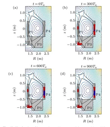
Fig.13. The fraction of lost passing and banana particles at position within the gray areas P1，P2，P3，and P4 at different time in the case of perpendicular injection. The red“*”represents the lost passing particles and the blue“+”represents the lost banana particles. At 900 Tic， the fraction of lost passing particles at P1， P2， P3， and P4 is 0.37%， 11.79%， 0%， and 67.25% respectively，while the fraction of lost banana particles at P1，P2，P3，and P4 is 0%，0%，0%，and 20.58%respectively.

To investigate the impact of collisions on lost particles，we use ISSDE to track each particle until the lost moment.The distribution of the initial time and the lost time of each lost particle with energiesE1，E2，andE3caused by Coulomb collisions in thePζ–Λspace is shown in Fig. 14. Because of the collision， the lost particle position in thePζ–Λspace greatly changes. We can divide these changes into two cases.One is that the lost particle position in thePζ–Λspace changes from the confinement region to the loss region， and the other is that the particles are still in the confinement region，but the particles are still lost. For these two cases， we both select 4 particles in the perpendicular injection beam with energyE1from Fig. 14 and draw their orbits in the position space. We show the selected particles in Fig. 15， and the corresponding particle orbits in Figs.16 and 17. In Fig.15，the blue“*”and“o”represent the case one， and the red“*”and“o”represent the case two. In Figs. 16 and 17， the black “*” shows the fast ion loss position under the impact of the collision. Because these particles are close to the minimum magnetic field strength boundary of the LCFS in thePζ–Λspace，they will be lost near the weak field side of the midplane under the effect of collision. The trajectory in the position space is not much different from case one to case two. These data suggest that when we consider the pitch-angle scattering loss of fast ions caused by Coulomb collisions，the distribution inPζ–Λspace may not give all the losses，and the particle trajectory evolution information is still needed.

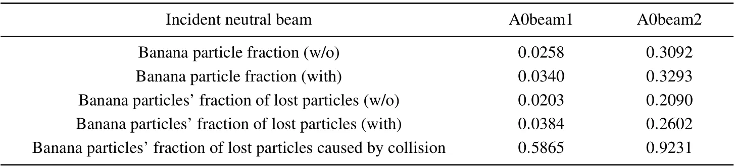
Table 3. The fraction of fast ion loss，banana ions with and without(w/o)Coulomb collision.

Fig.14. The distribution of lost ions caused by Coulomb collisions in the tangential beam and perpendicular beam in Pζ–Λ space at different times. The blue dot represents the position at the initial time，and the red circle represents the position at the lost time of each particle.

Fig. 15. The distribution of several typical particles from Fig. 14(a) for the perpendicular beam，which is numbered 1–4.The blue and red represent case one and case two.Case one is that the lost particle position in the Pζ–Λ space changes from the confinement region to the loss region，and case two is that the particles are still in the confinement region，but the particles get lost.

Compared with the prompt loss on a short timescale，the loss caused by Coulomb collisions is on a long timescale and has a continuous effect. Extending the calculated total time to 5.85×106Tic， we get the particle loss graph as shown in Fig.18. Compared with the loss rate of prompt loss， the loss rate caused by Coulomb collisions is smaller. We assume that the average background particle temperature is 2.3 keV， and the incident particles with energies greater than 3/2 the average background particle temperature are fast ions. Excluding lost particles caused by the prompt loss，within 5.85×106Tic，the additional fast ion losses caused by Coulomb collisions of tangential beams and perpendicular beams accounted for 16.21%and 25.05%of the total particles，respectively. The results are in agreement with the trend of the results calculated by the guiding-center orbit program GYCAVA under similar conditions. As shown in Fig.8 in Ref.[41]，the inconsistency in the numerical magnitude of the results stems mainly from the difference in the equilibrium magnetic field.Under the combined action of magnetic drift and Coulomb collisions， the lost position of most particles lost caused by Coulomb collisions are at P4， as shown in Fig. 19. The initial position distribution of the fast ion loss caused by Coulomb collisions is shown in Figs.19(b)and 19(d).Interestingly，compared with the prompt fast ion loss as shown in Figs. 7 and 8(c)， most of the lost fast ions caused by Coulomb collisions are concentrated on the low-field side，and there are more fast lost ions around the region far from the LCFS. Coulomb collisions cause the loss through the stochastic diffusion of fast ions and the pitch-angle scattering. We can see the change of the average areal density distribution， as shown in Figs. 20 and 21. After the prompt loss occurs， most of the fast ions are confined in the plasma center. Under the effect of Coulomb collisions， pitch-angle scattering happens. Some particles close to the LCFS will suffer the pitch-angle scattering loss，while the particles far from the LCFS will undergo a diffusion process formed by multiple pitch-angle scattering.During the diffusion process，some part of the fast ions gradually approach the LCFS and are eventually lost，and the other part of the fast ions become the thermal ions.

Fig.16. The typical particle trajectory in the case one corresponding to 1–4 as shown in Fig.15.

Fig.17. The typical particle trajectory in the case two corresponding to 1–4 as shown in Fig.15.

Fig. 18. When the total time is 5.85×106 Tic， the fast ion loss evolution under the impact of Coulomb collisions，the blue and red solid lines show the fast ion loss of the tangential and the perpendicular injection beam on the FW boundary. The blue and red long dashed lines show the prompt loss of the tangential and the perpendicular injection beam on the FW boundary when there is no collision.The results are consistent with that of Fig.8 in Ref.[41].

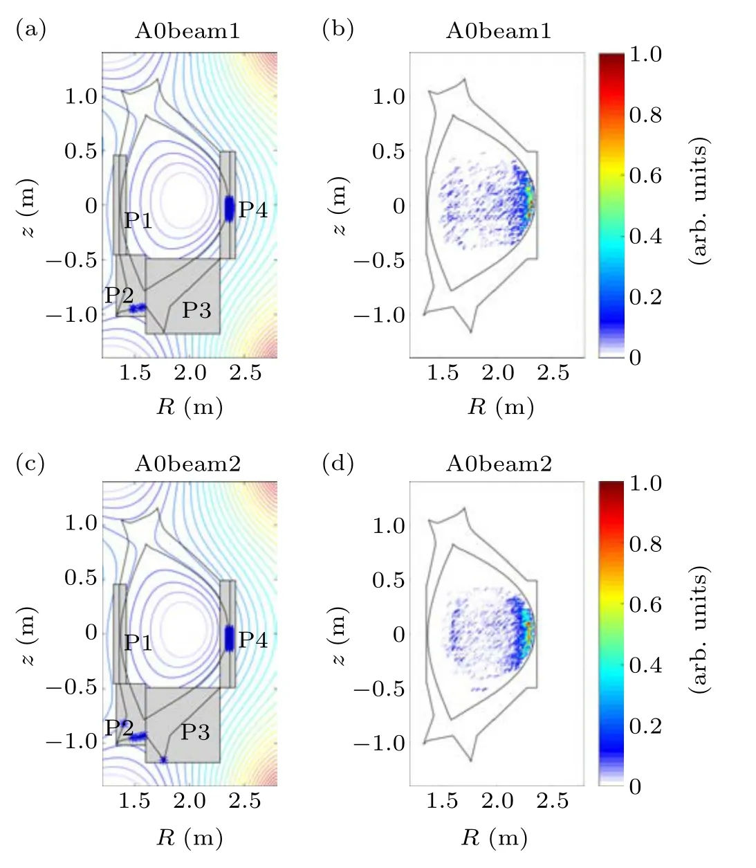
Fig. 19. Excluding the prompt loss， the position of and fraction of fast ion loss caused by Coulomb collisions and the initial distribution of the lost fast ions. Panels (a) and (b) are the case of tangential injection beam， and panels(c)and(d)are the case of perpendicular injection beam. The gray square area represents the position of the FW below the midplane. In panel (a)，the final fast ion loss caused by Coulomb collisions at P4 accounts for 6%of total tangential injection ions. In panel (c)， the final fast ion loss caused by Coulomb collisions at P4 accounts for 13.22%of the total perpendicular injection ions.

3.3. Fast ion slowing down in EAST

The slowing down process of fast ions will heat the background plasma. We can divide the ensemble average evolution of the physical quantities of fast ions into two stages，the velocity space diffusion stage and the slowing down stage.The ensemble average evolution of velocity and energy of fast ions in the slowing down process calculated by ISSDE can be shown in Figs. 22 and 25. In 8×104Tic， the ensemble average velocity and energy of the fast ions oscillate under the influence of the toroidal magnetic field，and the ensemble average kinetic energy of the ions is transferred in parallel and perpendicular directions. The total ensemble average kinetic energy of the ions decreases slightly due to the different loss rates of ions with different initial energies.More fast ions with the 65.224 keV and 65.644 keV have been lost as shown in Fig.11.Under the effect of the collision，the ensemble average velocity and energy of the fast ions will become equilibrium.Under the effect of the Coulomb collision，the ensemble average velocity and energy of the fast ions will reach equilibrium.Compared to the tangential injection，the perpendicular injection takes longer to reach equilibrium because the fraction of banana ions is higher in the perpendicular injection.More ions will bounce and the velocity space diffusion takes longer.

Fig.20. Average areal density distribution of tangential injection beam fast ions at different moments.

We can also see the diffusion from the particle distribution in the velocity space， as shown in Figs. 23 and 24. At the initial moment， the tangential and perpendicular injection beams are anisotropic collections of particles with three energies in velocity space. We use red， blue， and black to represent 1/3 total energy， 1/2 total energy， and total energy particles. On short timescales， such as 150Tic， the magnetic field will mainly affect the motion of fast ions in velocity space. In this process，the phase difference of the fast ions in the velocity space becomes larger and larger， and stochastic diffusion occurs in the velocity space. In the range of 1000Tic，the energy of fast ions hardly varies because the characteristic time of Coulomb collisions is three orders of magnitude longer than the ion cyclotron period.And the velocity diffusion of ions under a magnetic field occurs on a fixed sphere in velocity space.The evolution of the ensemble average energy of the fast ion is shown in Fig.25.

Fig. 21. Average areal density distribution of perpendicular injection beam fast ions at different moments.

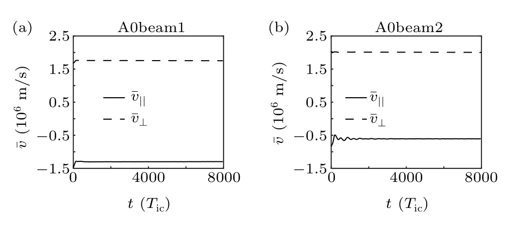
Fig.22. Evolution of the ensemble average velocity of fast ions.

Since the timescale of the velocity space diffusion stage is very short，the slowing down process cannot be seen. When we set the total number of time steps to 5.85×106Tic， we obtain the evolution of the ensemble average energy and velocity， as shown in Figs.26 and 29. In Fig.26， the ensemble average parallel velocity of the tangential and perpendicular injection beams gradually approaches 0 m/s under the effect of Coulomb collisions.

The evolution of the fast ion ensemble in parallel and perpendicular velocity space is shown in Figs. 27 and 28. The parallel and perpendicular velocity distribution functions of the tangential and perpendicular injection beams broaden under the effect of Coulomb collisions. Under the influence of Coulomb collisions， the spherical radius of velocity space decreases when fast ions transfer energy to the background plasma. In Fig.29，we can see that the energy of the tangential and perpendicular injection beams decreases in all directions and tends to the equilibrium value.

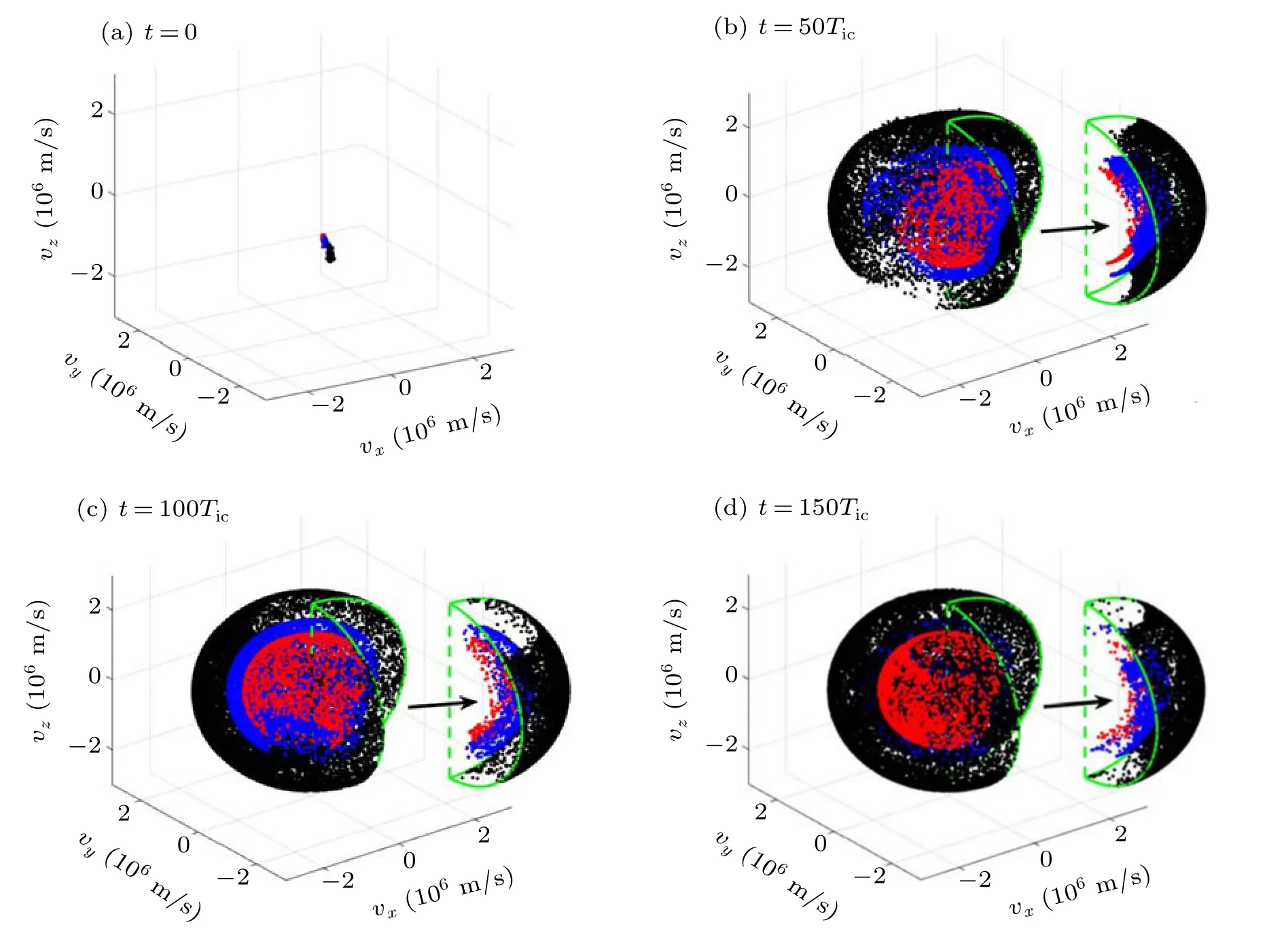
Fig.23. Evolution of fast ion distribution of tangential injection in velocity space at the velocity space diffusion stage.

Fig.24. Evolution of fast ion distribution of perpendicular injection in velocity space at the velocity space diffusion stage.

Fig.25. Evolution of the ensemble average energy of fast ions.

Fig.26. The evolution of the average velocity of the fast ion as the total time is 5.85×106 Tic.

Fig.27. Evolution of fast ion distribution of tangential injection in velocity space for large timescale.

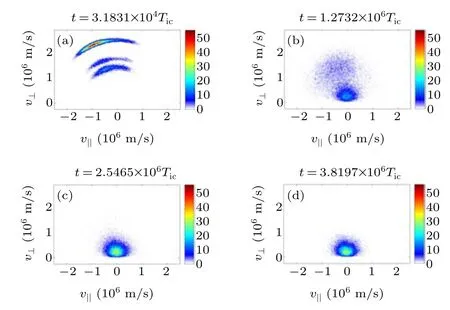
Fig.28. Evolution of fast ion distribution of perpendicular injection in velocity space for large timescale.

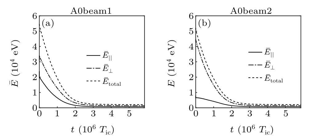
Fig.29. The evolution of the average energy of the fast ion as the total time is 5.85×106 Tic.

4. Conclusion

In this paper，we use the implicit Monte–Carlo full-orbitfollowing parallel program ISSDE to calculate the prompt loss and slowing down of NBI fast ions in EAST in the equilibrium configuration.We use EFIT to calculate the plasma parameters in the equilibrium configuration， while NUBEAM estimates the initial distribution of NBI fast ions. Simulation results show that it is more realistic to use the FW boundary to define the prompt loss of fast ions compared to the LCFS boundary，especially for fast ions with large radius of gyration.More ions drift out of the LCFS and return to the LCFS in the perpendicular injection beam than in the tangential injection beam， so the use of prompt loss with FW boundary is more relevant for the perpendicular injection beam.When considering Coulomb collisions， the marginal particles undergo pitch-angle scattering losses.

The ratio of the prompt loss rate and orbital type of fast ions depends on the initial distribution of fast ions inPζ–Λspace. The fraction of banana particles among the ions lost due to Coulomb collisions is very high. For the perpendicular beam， this fraction of particles is 92.31%. For the tangential beam， when banana particles account for 2.58% of the total number of particles， the proportion of banana particles in the lost particles due to collisions still reaches 58.65%.Coulomb collisions continuously affect the fast ion loss in long timescale simulations. Pitch-angle scattering and stochastic diffusion play an important role in the fast ion loss due to Coulomb collisions. We divide the slowing down of fast ions into the velocity space diffusion and the slowing down stage.The fast ions exchange momentum and energy with the background plasma through Coulomb collisions and transfer energy to the background plasma.

Not only for the NBI fast ions，the slowing down and energy deposition of alpha particles produced by nuclear fusion can also be calculated by ISSDE when the initial time velocity and position distribution are given. The collision crosssection will be smaller because the alpha particle energy is higher，and the corresponding collision coefficient will be different. The long time effect of Coulomb collisions on the loss of fast ions is not negligible， and the fast ions become loss particles or thermal particles under the effect of Coulomb collisions.Considering the total energy loss due to fast ion losses，we can more accurately calculate the momentum and energy transferred to the background plasma by collisions during the slowing down of the fast ions. Because the beam ion loss measurement[42]and triton burnup measurement[43]on EAST is still under development， we will provide experimental and numerical comparison results in future research work.

ISSDE is a test particle orbit-following parallel simulation program with Coulomb collisions. It can calculate the dynamic behavior of simulated particles under various external fields and disturbances， especially for simulating multiscale and multi-degree-of-freedom physical problems. However，we have not considered the effect of self-consistent fields.The PIC program with kinetic theory of collisions can provide more information， especially when particle losses caused by microscopic instabilities of the plasma need to be considered，which we will present in future work. The causes of fast ion losses on the actual EAST are multiple and complex，such as magnetic ripple losses， losses due to unstable magnetic fluid modes，losses due to resonant magnetic perturbation coils，and losses due to unstable modes. We will investigate the different effects of Coulomb collisions on these loss mechanisms in future work.

Acknowledgments

Project supported by the National MCF Energy Research and Development Program (Grant No. 2018YFE0304100)，the National Key Research and Development Program of China (Grant Nos. 2016YFA0400600， 2016YFA0400601，2016YFA0400602， and 2019YFE0302004)， and the National Natural Science Foundation of China (Grant Nos. 11805273 and 11905220). One of the authors (Yifeng Zheng) thanks Feng Wang and Shijie Liu from Dalian University of Technology for the benchmark work with PTC. Numerical computations were performed on Tianhe High Performance Computing Cluster in National Supercomputer Center in Tianjin.