
Optimal Control of Heterogeneous-Susceptible-Exposed-Infectious-Recovered-Susceptible Malware Propagation Model in Heterogeneous Degree-Based Wireless Sensor Networks
2022-08-08 05:47ZHANGHongSHENShigen沈士根WUGuowen吴国文CAOQiying曹奇英XUHongyun许洪云
关键词:吴国
ZHANG Hong(张 红), SHEN Shigen(沈士根), WU Guowen(吴国文),CAO Qiying(曹奇英), XU Hongyun(许洪云)
1 School of Computer Science and Technology, Donghua University, Shanghai 201620, China 2 Department of Computer Science and Engineering, Shaoxing University, Shaoxing 312000, China 3 Faculty of Business Information, Shanghai Business School, Shanghai 201400, China
Abstract: Heterogeneous wireless sensor networks(HWSNs)are vulnerable to malware propagation, because of their low configuration and weak defense mechanism. Therefore, an optimality system for HWSNs is developed to suppress malware propagation in this paper. Firstly, a heterogeneous-susceptible-exposed-infectious-recovered-susceptible(HSEIRS)model is proposed to describe the state dynamics of heterogeneous sensor nodes(HSNs)in HWSNs. Secondly, the existence of an optimal control problem with installing antivirus on HSNs to minimize the sum of the cumulative infection probabilities of HWSNs at a low cost based on the HSEIRS model is proved, and then an optimal control strategy for the problem is derived by the optimal control theory. Thirdly, the optimal control strategy based on the HSEIRS model is transformed into corresponding Hamiltonian by the Pontryagin’s minimum principle, and the corresponding optimality system is derived. Finally, the effectiveness of the optimality system is validated by the experimental simulations, and the results show that the infectious HSNs will fall to an extremely low level at a low cost.
Key words: heterogeneous wireless sensor network(HWSN); malware propagation; optimal control; Pontryagin’s minimum principle
Introduction
Heterogeneous wireless sensor networks(HWSNs)are a kind of wireless sensor networks(WSNs),composed of a great many of resource constrained and heterogeneous sensor nodes(HSNs)to detect physical environmental conditions.These HSNs have different computing resources, energy, and communication, and that HWSNs have the advantages of strong pertinence, high flexibility, and low cost[1].With these characteristics, HWSNs thus have been deployed in many practical applications, such as smart life, biological medicine, environmental monitoring, and military[2].
In HWSNs, there exists the failure of HSNs caused by malware, which is an application with malicious intent, ruining the normal work of HWSNs by injecting malicious data, blocking communication channels, or occupying computing units.Besides, the HSNs systems have no strong hardware and software with limited resources, which make the defense mechanism weak, so that the malware in HWSNs is prone to propagation[3-4].To solve this problem, many researchers have studied the methods and processes of malware propagation in HWSNs.For example, Illiano and Lupu[5]presented many methods of malicious data injection in WSNs.Ho[6]presented on demand software-attestation based scheme to defend against worm propagation in WSNs.
The propagation process of malware in HWSNs is similar to that of diseases in human populations[7], and thus epidemiology is commonly applied to study malware propagation.The classic epidemic models include susceptible-infectious(SI), susceptible-infectious-susceptible(SIS), and susceptible-infectious-recovered(SIR)[8-10].In this paper, we propose a heterogeneous susceptible-exposed-infectious-recovered-susceptible(HSEIRS)model, containing statesS,E,I,Rto describe all the states of HSNs infected by malware.We add the statesEandSto the classical epidemic model SIR.Because some malware may have an incubation period in reality.That is to say, when HSNs are infected by malware, they may propagate malware to other HSNs with delay.Besides, when the recovered HSNs encounter unknown malware, they usually lack of immunity, and thus the state will change fromRtoS.
There are generally two ways to solve the problem with malware propagation in HWSNs.One is based on the qualitative analysis[11-13], such as proving the existence of equilibrium points and attaining the basic reproduction number governing the stability of the equilibrium points; the other is based on the optimal control theory[14-17], which is defined by an optimal strategy to achieve a low level of infectious HSNs at a low cost.The second way is more suitable for solving the problem of active defense malware propagation in HWSNs.In this paper, we thus apply it to suppress malware propagation in HWSNs by defining a dynamic optimal control strategy.Using the communication channels of HWSNs, the patches corresponding to malware can be sent to some infectious HSNs to defend their systems, which are effective in enhancing the overall defense capability of HWSNs.
Our contributions are summarized as follows.
(1)An HSEIRS model is proposed, which is the major work to describe the state dynamics of HSNs in HWSNs.
(2)The existence of an optimal control problem based on the HSEIRS model is proved, and then an optimal control strategy for the problem is derived using the optimal control theory.
(3)Using the Pontryagin’s minimum principle, the optimal control strategy based on the HSEIRS model is transformed into the corresponding Hamiltonian, and an optimality system based on the HSEIRS model is derived.
The difficulty of this paper lies in proving the existence of an optimal control problem based on the HSEIRS model, and deriving the optimality system based on the HSEIRS model.
The rest of the paper is presented as follows.In section 1, the related works are reviewed.In section 2, an HSEIRS model is proposed.In section 3, an optimality system based on the HSEIRS model is derived, and the theoretical analysis of the optimization problem is presented.In section 4, a calculation algorithm is presented to validate the optimality system and the results of data analyses are also shown using the relevant parameters.Finally, the conclusions of the paper are given.
1 Related Works
Many researchers have illustrated various extended epidemic models for WSNs.For example, a susceptible-exposed-infectious-susceptible-recovered-vaccination(SEIRSV)model containing the statesS,E(exposed),I,R, andV(vaccination)[18]; a susceptible-infected-immunized(SII)model[19]; a worm propagation model considering the spatial-temporal perspective[20]; a susceptible-active-dormant-immune(SADI)model considering the hierarchical topology structure[21]; and a susceptible-infected-susceptible-vaccinated(SISV)model[22].
Furthermore, various methods have been presented to solve the problems with malware propagation in WSNs.Liuetal.[23]used the stochastic game to propose a method for WSNs to predict the probability of malware adopting the spread behavior.Shenetal.[24]developed traditional epidemic theory and constructed a malware propagation model by differential equations to represent the dynamics between states.They considered HWSNs and set up a dependability assessment mechanism for HWSNs with malware propagation[25].They also considered a clustered WSNs under epidemic-malware propagation conditions[26].Jiangetal.[27]established a new attack-defense game based on Stackelberg game.Acaralietal.[28]thought of the epidemic modeling to the Internet of things(IOT)networks consisting of WSNs.Wangetal.[29]proposed a method using the pulse differential equation and the epidemic theory for WSNs preventing from malware propagation.Shenetal.[30]proposed a malware detection infrastructure realized by an intrusion detection system(IDS)with cloud and fog computing to preserve the privacy of smart objects in the IOT networks and suppress malware propagation.
In addition, some researchers have applied the optimal control theory to study the infected networks.Zhangetal.[31]proposed a time-varying control mechanism of an SIQRS epidemic model of the network in terms of vaccination, quarantine and treatment by the optimal control theory.Xuetal.[32]proposed a novel SIVRS mathematical model for epidemic spreading based on complex networks, where an optimal control problem was formulated to maximize the recovered agents with the limited resource.Dongetal.[33]presented a general formulation for the optimal control problem to a class of fuzzy probability differential systems relating to SIR and SEIR epidemic models.Darajatetal.[34]discussed an optimal control on the spread of SLBS computer virus model.Zhang and Huang[35]solved an optimal control problem for the combined impact of reinstalling system and network topology on the spread of computer viruses based on scale-free networks.Ganetal.[36]proposed a novel dynamical model with an external compartment to control the level of infected computers based on the optimal control theory.Bietal.[37]addressed the development of a cost effective dynamic control strategy of disruptive viruses.Yangetal.[38]presented the optimal control problem for capturing the optimal dynamical immunization based on a controlled heterogeneous node-based SIRS model.
The dynamical optimal control strategy based on HWSNs has not been worked out yet.The first issue is how to characterize the feature of HSNs in infected HWSNs; the second issue is how to formulate the optimal control problem with installing effective antivirus programs for infectious HSNs.Here, we focus on the first issue by proposing an HSEIRS model based on epidemiology.After that, we handle the second issue by deriving the optimality system based on the Pontryagin’s minimum principle, which is proved to be effective by experimental simulations and data analysis.
2 Description of HSEIRS Model
From the perspective of network topology, HSNs are divided into two categories.One is data nodes randomly distributed in the detection area, which are responsible for collecting and transmitting data; the other is gateway nodes, which are responsible for aggregating data and transmitting control information.Obviously, the gateway nodes are better than the data nodes in terms of the processing capacity, storage capacity and calculation capacity.In this paper, we characterize HSNs on the basis of the heterogeneity of the degrees.According to the degree number of an HSN, they are divided intoMgroups, whereMmeans the number of HSN groups, the HSNs have the same degree in each group.For simplicity, we identify the degree of HSN groupi∈{1, 2, …,M} withi∈{1, 2, …,M}, and letSi(t),Ei(t),Ii(t), andRi(t)be the probabilities of the HSN groupi∈{1, 2, …,M} in statesS,E,I, andRat timet, respectively.As shown in Fig.1, according to the degree of an HSN group, all HSNs can be divided into group 1, group 3 and group 4.

Fig.1 HWSNs topology
In terms of the other malware propagation models, we assume that the initial probability of HSN groupi∈{1, 2, …,M} in stateIisp,i.e.,
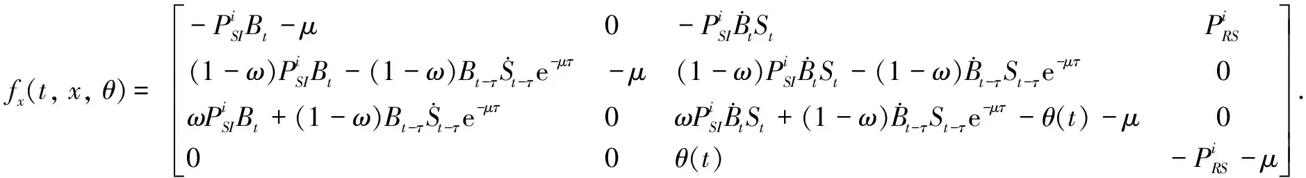
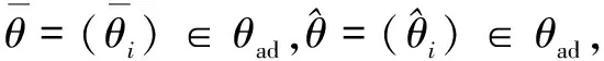
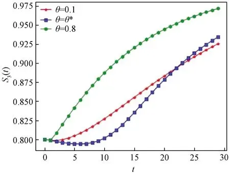
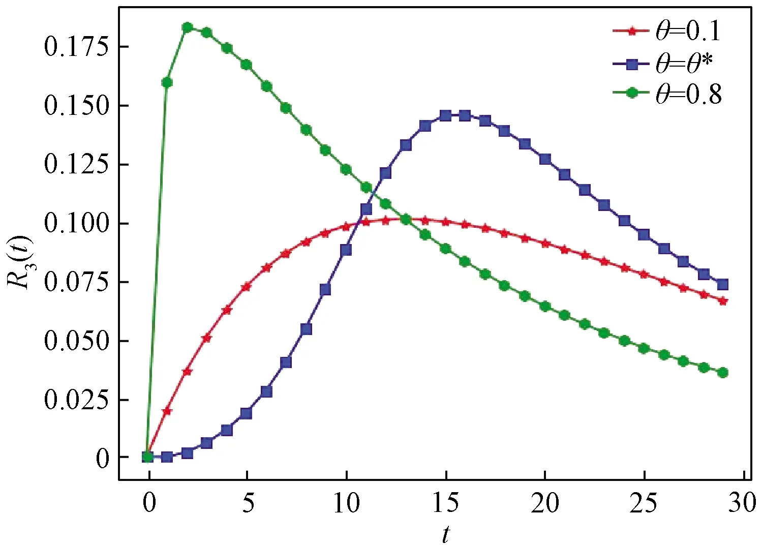
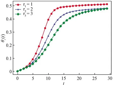
Ii(0)=p, 0 (1) We also assume that Ei(0)=Ri(0)=0. (2) In this manner, we obtain Si(0)=1-p. (3) (4) whereBi(t)denotes the probability of a susceptible HSN in groupiencountering infectious HSNs, (5) and (6) According to the characteristics of HSNs, we construct a state diagram about the behaviors of HSNs in HWSNs.In the state diagram, there is one state from five possible states at a certain time for an HSN.Specifically, if an HSN is in stateSat timet, it means that it is prone to being infected by malware but has not been infected yet; if it is in stateEat timet, it means that it has been infected by malware, but cannot propagate malware to its adjacent nodes by transmitting data or control information; if it is in stateIat timet, it denotes that it has been infected by malware and can propagate the malware to its adjacent nodes by transmitting data or control information; if it is in stateRat timet, it denotes that it is immune to malware.In addition, if it is in stateDat timet, it denotes that it loses all functions, as it has either entirely consumed its energy or been damaged by malware. Fig.2 State diagram for an HSN Motivated by the above, we propose the following HSEIRS model with delay timeτ, wherepdenotes the initial fraction of HSN groupiin stateI. (7) (8) (9) (10) subject to (11) In this section, the sufficient and necessary conditions of the optimal control strategy are presented. With regard to installing effective antivirus programs for infectious HSNs belonging to groupi, we adopt the central patch allocation strategy.An HSN in stateIbelonging to groupiis installed effective antivirus programs and becomes recovered with probabilityθi(t)per unit time.In order to describeθi(t)clearly, let us make some assumptions on theθi(t). (a)Fori∈{1, 2,…,M},θi(t)∈L2[0,tf]. (b)θi(t)is measurable. (d)Letθi(·)=(θ1(·),θ2(·),…,θM(·)). From these facts, we now consider an optimal control problem to minimize the objective function: (12) satisfying (13) subject to Si(σ)>0,Ei(σ)>0,Ii(σ)>0,Ri(σ)>0. (14) whereσ∈[-τ, 0]denotes the admissible time in the incubation period. In order to find an optimality system, we firstly find the Lagrange and Hamiltonian for the optimal control problem.In fact, the Lagrange of the optimal control problem is given by (15) whereξdenotes the cost of installing effective antivirus programs for infectious HSNs, and it is a small positive constant.To find the optimal control function for the optimal control problem, we define the corresponding Hamiltonian as (16) where (17) which are the adjoint functions of the optimal control problem. In order to prove the existence of an optimal control problem based on the HSEIRS model, six lemmas are established here. Lemma1 With regard to the optimal control problem(12), system(13)can be rewritten as (18) withx(t)∈Ω, wheref(t,x,θ)denotes the states function of the HSEIRS model, andΩis the positively invariant for system(13).The problem has an optimal control if the following five conditions are satisfied at the same time. (a)f(t,x,θ)is bounded by a linear function inx, the first partial derivatives are consecutive, and there is a constantZsuch that |f(t,x,θ)|≤Z, (19) |fθ(t,x,θ)|≤Z, (20) and |fx(t,x,θ)|≤Z(1+|θ|), (21) wherefθ(t,x,θ)is the first partial derivatives of the functionf(t,x,θ)toθ,fx(t,x,θ)is the first partial derivatives of the functionf(t,x,θ)tox. (b)There isθ(·)∈θadsuch that system(18)is solvable. (c)θadis convex and closed. One night, the girl caught ill. In moment of fluster9() , instead of calling her parents, she dialed the new boy s cell phone. The boy was already asleep but his cell phone was still on. (d)L(x,θ)is convex onθad. Next, we show the correctness of those five conditions by introducing and proving Lemmas 2-5. Lemma2f(t,x,θ)is bounded by a linear function inx, the first partial derivatives are consecutive, and there is a constantZsuch that systems(19)-(21)are satisfied. ProofFor simple description, the system(13)is rewritten as (22) We can obtain |f(t, 0, 0)|=|(μ0 0 0)T|, (23) (24) (25) Lemma3The system(18)is solvable. (26) Thus, the proof is complete. Lemma4θadis convex and closed. ProofLet (27) (28) and let 0<ε<1.SetL2[0,tf]denotes the control functionθi(t)which is integrable and bounded during the time period[0,tf].As(L2[0,tf])2Mis a real vector space, we get (1-ε)θ(1)(·)+εθ(2)(·)∈(L2[0,tf])2M. (29) So, the convexity ofθadfollows by the observation that, for 1≤i≤M, we have (30) Let θ(·)=(θ1(·),θ2(·),…,θM(·))T, (31) be a limit point ofθad, and let (32) be a sequence of points inθadsuch that (33) It comes from the completeness of(L2[0,T])2Nthat (34) So the closeness ofθadcomes from the observation that, for 1≤i≤M, we have (35) Thus, the proof is complete. Lemma5L(x,θ)is convex onθad. (36) Here, (37) (38) We can obtain (39) Thus, the proof is complete. ProofWe can chooseο1=ξ/2,ι=2.ο2is the lower bound onI, which is similar to that in Ref.[39].We can obtain (40) Further, (41) Thus, the proof is complete. ProofLemmas 2-6 show that the five conditions in Lemma 1 are all satisfied.Thus, the existence of the optimal control follows from Lemma 1. In this subsection, we present a necessary condition for the optimal control problems(12)and(13). (42) with transversality conditions (43) (44) ProofTo determine the adjoint equations and the transversality conditions, we differentiate the Hamiltonian, and obtain the adjoint system as (45) Thus, the adjoint system can be rewritten as system(42).By the optimal conditions, we have (46) From Theorem 2, we derive the following optimality system(47)and(48)for the optimal control problems(12)and(13). (47) and (48) Here, we validate the optimality system based on the HSEIRS model using Python.In our experiments, the HWSNs are composed of 1 000 HSNs,i.e.,M=1 000.The intervaltfis 10 time steps.We construct the HWSNs topology and set the experimental parameters referring to Ref.[40], the minimum degree of HSNs is 2, the maximum degree of HSNs is 20, and the mean degree 〈d〉 is 4. Using the forward and backward difference approximation, the calculation algorithm is described in Fig.3, where the step sizeh>0,τ=mh, andtf-t0=nh. Fig.3 Calculation algorithm to the optimality system based on the HSEIRS model Figure 4 shows the changeable probability trends of susceptible HSNs belonging to group 3 under different values of control variableθ.We observe different trends.Forθ=0.1,θ=θ*, andθ=0.8, the probabilities of susceptible HSNs gradually increase to 0.88, 0.88 and 0.95 in the first 22 time steps, respectively, these probabilities then slowly increase to 0.915, 0.925 and 0.975 after 8 time steps.Obviously, forθ=θ*, it has taken an effective control of the probability of susceptible HSNs. Fig.4 Changeable probability trends of susceptible HSNs under different values of control variable θ Figure 5 shows the changeable probability trends of infectious HSNs belonging to group 3 under different values of control variableθ.We observe different trends.Forθ=0.1,θ=θ*, andθ=0.8, the probabilities of infectious HSNs gradually decrease to 0.06, 0.06, and 0 in the first 13 time steps, respectively.These probabilities then slowly decrease to 0.025, 0, and 0 in the 20 time steps.Obviously, forθ=θ*, it has taken an effective control of the probability of infectious HSNs. Fig.5 Changeable probability trends of infectious HSNs under different values of control variable θ Figure 6 shows the changeable probability trends of recovered HSNs belonging to group 3 under different values of control variableθ.We observe some different trends.Forθ3=0.1, the probability of recovered HSNs gradually increases to 0.1 in the first 10 time steps, then slowly decreases to 0.075 in the 30 time steps.Forθ=θ*, the probability of recovered HSNs gradually increases to 0.15 in the first 15 time steps, then slowly decreases to 0.08 in the next 30 time steps.Forθ=0.8, the probability of recovered HSNs fast increases to 0.175 in the first 2 time steps, then slowly decreases to 0.04 in then 30 time steps.Obviously, forθ=θ*, it has taken an effective control of the probability of recovered HSNs. Fig.6 Changeable probability trends of recovered HSNs under different values of control variable θ Figure 7 shows the changeable probability trends of control variableθunder different values of delayτ.We observe some different trends.Forτ1=1,τ2=2, andτ3=3, the probabilities of control variableθgradually increase to 0.50, 0.43, and 0.38, respectively in the first 15 time steps, then slowly increase to a stable value.It can tell us that the optimal control variableθdeceases whenτincreases from 1 to 3. Fig.7 Changeable probability trends of control variable θ under different values of delay τ Figure 8 shows the changeable probability trends of control variableθunder different values.We observe different trends.Forθ=θ*, the probability of control variableθgradually increases from 0 to 0.5 in 30 time steps. Fig.8 Changeable probability trends of control variable θ under different values Figure 9 shows the changeable probability trends of control variableθunder different values of degreei.We observe different trends.Fori1=3,i2=10, andi3=20, the probabilities of control variableθgradually increase to 0.35, 0.50, and 0.80 in the first 15 time steps, respectively, then slowly increase to a stable value.It can tell us that the optimal control variableθincreases when the degreeiincreases from 3 to 20. Fig.9 Changeable probability trends of control variable θ under different values of degree i In this paper, we have studied an optimal control to malware propagation by installing effective antivirus programs for infectious HSNs in controlled HWSNs.We firstly proposed an HSEIRS model to describe the HSNs state dynamics of malware propagation in HWSNs, involving the exposed state and degree heterogeneity of HSNs.After that, we derived an optimality system to achieve a low level of infectious HSNs at a low cost based on the HSEIRS model through a series of theoretical analysis.Finally, using the forward and backward difference approximation, we validated the effectiveness of the optimality system by the calculation algorithm and data analyses.

3 Optimal Control Strategy Based on HSEIRS Model


3.1 Existence of an optimal control problem based on HSEIRS model


3.2 Optimality system based on HSEIRS model


4 Validating Optimal Control Strategy of HSEIRS Model


5 Conclusions
猜你喜欢
汽车实用技术(2022年16期)2022-08-31
小读者之友(2021年6期)2021-07-29
书香两岸(2020年3期)2020-06-29
上海采风月刊(2020年2期)2020-04-05
小天使·三年级语数英综合(2019年11期)2019-01-13
作文世界(小学版)(2018年7期)2018-10-16
当代贵州(2016年36期)2017-05-08
连环画报(2015年7期)2015-09-22
民间故事选刊·下(2015年3期)2015-03-09
领导文萃(2012年16期)2012-02-11
 Journal of Donghua University(English Edition)2022年3期
- Journal of Donghua University(English Edition)的其它文章
- Three-Dimensional Model Reconstruction of Nonwovens from Multi-Focus Images
- Toughness and Fracture Mechanism of Carbon Fiber Reinforced Epoxy Composites
- Three-Dimensional Metacomposite Based on Different Ferromagnetic Microwire Spacing for Electromagnetic Shielding
- Blockchain-Based Architectural Framework for Vertical Federated Learning
- Enhanced Arsenite Removal Using Bifunctional Electroactive Filter Hybridized with La(OH)3
- Students’ Feedback on Integrating Engineering Practice Cases into Lecture Task in Course of Built Environment