
UNDERSTANDING SCHUBERT'S BOOK (III)*
2023-01-09 10:57BangheLI李邦河
Banghe LI (李邦河)
KLMM,Academy of Mathematics and Systems Science,Chinese Academy of Sciences,Beijing 100190,China E-mail: libh@amss.ac.cn
Based on this one dimensional formula, Schubert was able to get all higher dimensional formulas by using only the multiplication of conditions.
We can see, however, that the definition of coincidence objects and the proof of formulas regarding these conditions are neither clear nor rigorous by modern standards.
After showing all the formulas regarding ε, Schubert gave the definition of complete coincident figures. He said:
“When we define the one dimensional condition ε, we assume that there is a determined line passing through two infinitely close points which is like two infinitely close points on a curve. However, if we regard each line in a bundle of lines, or more generally, each line in a cone as the connecting line passing through these two coincidence points and the coincidence point is the center of the bundle or the vertex of the cone, then we get a two dimensional coincidence condition. Finally, if we regard every line passing through the coincidence points as the connecting line, then we get a three dimensional coincidence condition, or a complete coincident figure.”
This definition is, unfortunately, difficult to understand.
Schubert then gave proofs for a few forms of Bezout’s theorem, as an application of the coincidence formulas he had just obtained.
In this paper,we try to give a rigorous description of Schubert’s ideas,including explaining the definition of coincidence conditions and the proofs of these coincidence formulas in such a way that satisfies the standards of modern mathematics. In Section 2, we show the exact space in which Schubert actually worked, so that we can easily identify what his conditions really were. Then, we prove all the coincidence formulas in §13 of his book following his ideas.In Section 3, we give a few comments about Schubert’s ideas, pointing out the validity and limitations of these ideas. We also provide a proof of Bezout’s theorem using the modern theory of Chow rings. In Section 4,we give an application of the coincidence formulas following Schubert’s path. Schubert gave a second method for calculating the number of curves in one dimensional planar systems that are tangent to a given planar curve in §14 as an application of the coincidence formulas. For a planar curve of degree m and rank n, the number is nµ+mν.To calculate this number, we should give a precise definition for a system of planar curves. To avoid ambiguity, we also give the precise definition of dual curves. Based on this, we define the system of planar curves. In [3], we assumed that for the nonempty Zariski open set of a one-dimensional system, the curves are irreducible, and the dual curves have the same rank.We prove here that the same degree must imply the same rank for any system. Finally, along the lines of Schubert’s ideas,we provide a rigorous proof that the number is nµ+mν. A natural question to ask is: can any curve of degree m and rank n define a condition in any system of planar curves? We give an affirmative answer to this question in Section 5.
2 Coincidence Formulas for Pairs of Points
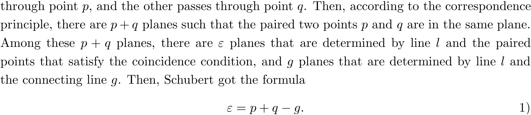
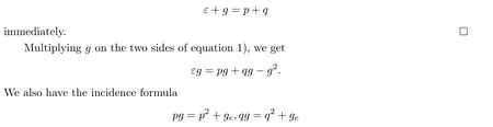
Let π1×π2×π3: B3→CP3×CP3×G(3,1) be the natural projection. Then in the formula of Schubert
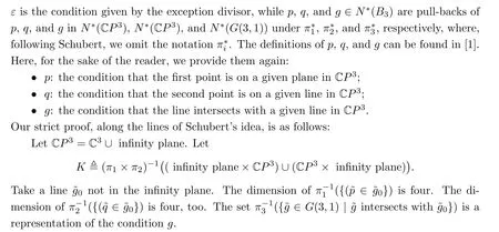
Choose the coordinate (p1,p2,p3) ∈C3such that ˜g0∩C3is given by the equation p1=p2= 0. Thus all the planes passing through ˜g0are given by the equation p2= ap1, where a ∈C ∪{∞}=CP1.
To give the coordinates of B3,we first give the coordinates of C3×C3,(p1,p2,p3,q1,q2,q3).Change the coordinates to (p1,p2,p3,u1,u2,u3), where

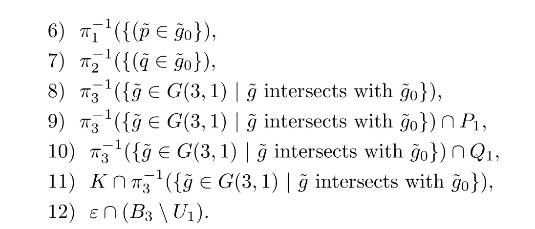
According to condition 1), for s ∈γ, there are at most finite s ∈K. Thus, with the exception of finite points, p1(s), p2(s), p3(s), q1(s), q2(s) and q3(s) are well defined in C, s ∈γ.According to conditions 9) and 10), p1(s) and p2(s) and also q1(s) and q2(s) are not both zero.Let p2(s)=a(s)p1(s), q2(s)=b(s)q1(s), a(s),b(s)∈CP1. For the finite points in K, according to conditions 6) and 7), p(s),q(s) are not on the line ˜g0, so the plane that passes through p(s)and ˜g0and the plane that passes through q(s) and ˜g0are uniquely determined, which then determines an element in CP1×CP1. Thus, we have the morphism of γ to CP1×CP1.
Then we need only consider the case that (a(s),b(s)) forms a curve in CP1×CP1. For the mapping sa(s), with the exception of finite points in CP1, the inverse of this mapping has the same number of points. This number is just p([γ]). The same applies for q([γ]).
If, for all s ∈γ, we have that a(s) = b(s), then p(s) and q(s) are in the same plane that passes through ˜g0. Thus, there are infinite lines passing through p(s),q(s) and ˜g0, and this contradicts the condition 8). Therefore, there are only finite s ∈γ such that a(s)=b(s).
For s ∈γ such that a(s) = b(s), there are two possibilities. One is that p(s) /= q(s).According to condition 11), both p(s) and q(s) are in C3. The other possibility is that p(s) =q(s). According to condition 3), p(s)=q(s)∈C3.
Now we look at the multiplicity. The equation of the diagonal is
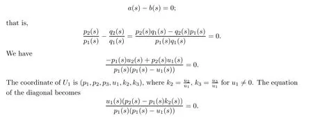
Assume that s0∈γ such that a(s0)=b(s0). According to conditions 4), 5), 9)and 10), we know that p1(s0)/=0, q1(s0)/=0.
Then,u1(s0)=0 represents the fact that s0is in ε,and p2(s0)-p1(s0)k2(s0)=0 represents the fact that s0satisfies the condition g.
Fix a branch of γ at s0. Represent elements in γ near s0in this branch by a parameter t in a neighborhood of 0 belong to C, which is denoted by s(t). Substituting s with s(t) in the equation of the representation of the diagonal, we get
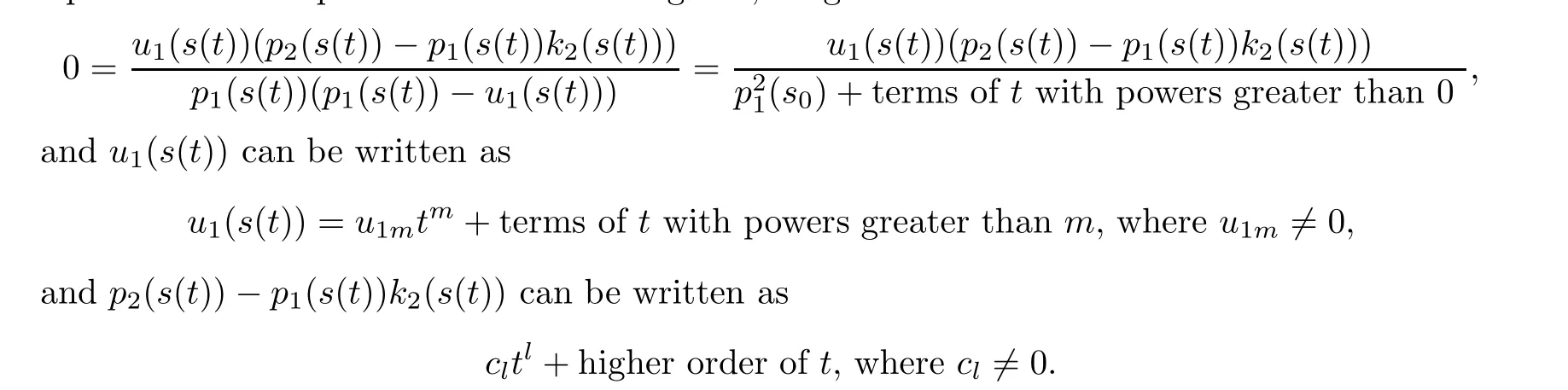
The multiplicity of s0in ε in this branch is m, and the multiplicity of s0satisfying condition g in this branch is l.
Therefore, the number of elements in γ satisfying a-b = 0 with multiplicity is equal to ε[γ]+g[γ].
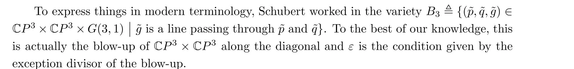
Remark For n ≥2, let Bnbe {(˜p,˜q,˜g) ∈CPn×CPn×G(n,1) | ˜g is the line passing through ˜p and ˜q}, where G(n,1) is the Grassmann variety formed by the lines in CPn. Then Bnis the blow-up of CPn×CPnat the diagonal. Let ε be the exception divisor and let g be the condition given by all lines in CPnintersecting with a given n-2 dimensional subspace of CPn. Then the above proof gives
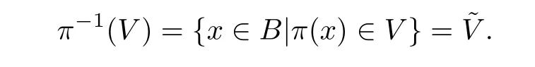
Lemma 2.1 Let B be the blow-up of X along Y, where X,Y are nonsingular varieties.π is the natural projection from B to X. V is a subvariety of X intersecting Y properly. The strict transformation ˜V of V is the closure of π-1(V Y) in B. Then,
Proof Let X be the variety of dimension n, let Y be the variety of dimension m, and let V be the variety of dimension k. Here m ≤n-2. As V intersects Y properly,the dimension of V ∩Y is m+k-n. If V ∩Y is empty, there is nothing to do, so we assume that m+k-n ≥0,and V ∩Y is nonempty.
There are finite components of V ∩Y. Let Y1be one of its components. The dimension of π-1(Y1) is (m+k-n)+(n-m-1)=k-1. For any y ∈Y1, as V intersects Y properly, we can find a sequence vi∈V Y, i = 1,2,... such that vi→y as i →∞. Thus we can find a subsequence of videnoted by wisuch that π-1(wi) converges to a point ˜y ∈B with π(˜y)=y.Because ˜V ∩π-1(Y1) is a component of ˜V ∩π-1(Y) and the dimension of ˜V ∩π-1(Y) is at least k-1, the dimension of ˜V ∩π-1(Y1) is at least k-1. On the other hand the dimension of π-1(Y1) is k-1, so the dimension of ˜V ∩π-1(Y1) is k-1. Thus, ˜V =π-1(V). □
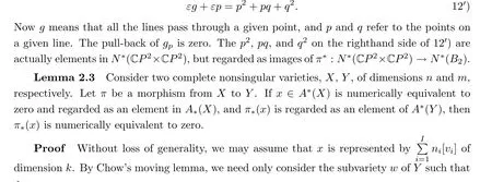
Lemma 2.2 Let B be the blow-up of X of dimension n along Y, where X,Y are nonsingular varieties. π is the natural projection from B to X, which is proper. Thus π∗is a well defined map from A∗(B) to A∗(X). For any element x ∈Ak(X), regard π∗(x) ∈A∗(B) as elements in A∗(B). Then,
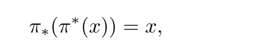
where π∗(π∗(x))∈A∗(X) is regarded as an element in A∗(X).
Proof By Chow’s moving lemma,we may assume that x is represented by a subvariety V of X which intersects Y properly. Then, π∗(x)=π-1([V]). The monomorphism π :π-1(V)→V is of degree one, so
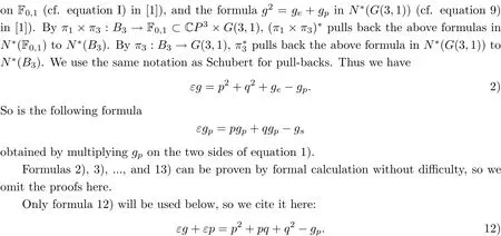
After formula 13), Schubert said “According to 12), we can obtain the correspondence principle on a plane published first by Zeuthen”. Actually,to prove the correspondence principle on a plane, we have to work in B2. By the natural inclusion B2⊂B3, formula 12) is pulled back to N∗(B2), which leads to

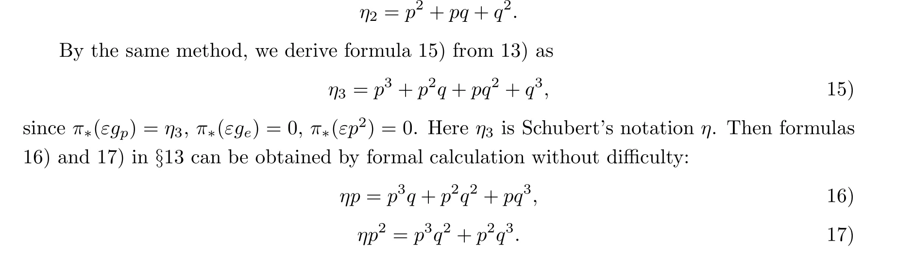
Denote the condition of the diagonal in CP2×CP2by η2. Thus, π∗(εg) = η2. As π(εp) is a one-dimensional subvariety of the diagonal,π∗(εp)=0. Moreover,by Lemma 2.2,π∗(p2)=p2,π∗(pq)=pq, π∗(q2)=q2. To summarize, the correspondence principle on a plane is
After these formulas, Schubert proved Bezout’s theorem for dimension three. He said:
“Given two point systems, we combine every point in one system to any points in the other to get a point pair system consisting only of complete coincidence objects. Assume the given two point systems are surfaces of degree m and n, respectively (that is, two two-dimensional point systems). Then, the righthand side of equation 16) is reduced to p2q2. This item is actually mn, for the line determined by p2would intersect the surface of degree m at m points and the line determined by q2would intersect the surface of degree n at n points. So there are mn pairs of points, and then there is a point pair system of dimension four. So formula 16)infers the following important Bezout’s theorem:
‘The degree of a curve obtained by intersection of two surfaces is the product of the degrees of these surfaces.’
Similarly, according to 15) or 14), we can get the next theorem:
‘The intersection of a surface of degree m and a curve of degree n is mn points.’
The above two theorems lead to the following theorem:
‘The intersection of three surfaces of degree m,n and l, respectively, is mnl points.’ ”
3 Comments
1. Schubert’s starting point is the set whose element is a line in CP3with two points; this starting point prevents people realizing that it is actually a blow-up of CP3×CP3.
2. When Schubert described that two points are infinitely closed,he was considering the line connecting these two points. The term coincidence figure means that on the line the two points are coincident. When he used the term complete coincidence, he meant that two points are coincident and no lines are involved. To give a rigorous description, Schubert’s use of infinite closeness is better being replaced by nonstandard analysis. In the language of nonstandard analysis, let∗CP3be the nonstandard extension of CP3. Two points in∗CP3are infinitely close if and only if they are in the monad of the same point in CP3. The line connecting these two points are elements in∗G(3,1), whose standard part in G(3,1) is a line in CP3passing through standard points. This line, together with the points regarded as coincident points,is an element in B3. Now it is clear that the complete coincident figure is an element in the diagonal of CP3×CP3. Thus, the coincident figure and the complete coincident figure are different things in different spaces. Readers can also refer to Kleiman’s paper [4], which gives an intuitive explanation of complete coincidence.
3. How do we understand Schubert’s words after formula 17): “Note that these formulas can only be used in the system that only contains complete coincident figures (cf. the last paragraph in §5).” ? Furthermore, in the last paragraph in §5, he said:
“For figures with c parameters, we also consider this kind of equation of dimension α that would hold only when all the conditions of dimension α in this equation add some special kind of condition of dimension c-α. In other words, the equation does not hold for every system of dimension α, but only holds for some special kind of system of dimension α. So, it is very natural that we need to indicate the scope of the validity of any equations, and when we apply condition z to symbol multiplication, we must check whether condition z is in the scope of the validity of this system. If a formula of dimension α is valid for all systems of dimension α,we say that it generally holds. For the examples that hold only for special systems but not generally, see §13 formula 14) to 17) and formulas in §25 and §26.”
From Schubert’s words above we see that when he said that the formula holds generally,he meant that it holds in N∗(B3). When he said that formulas 14) to 17) can only be used in the system of complete coincident figures, he meant that they hold in π∗(N∗(CP3×CP3)) ⊂N∗(B3). By Lemma 2.2, π∗:N∗(CP3×CP3)→N∗(B3) is a monomorphism. Thus Schubert correctly regarded N∗(CP3×CP3) as a subset of N∗(B3). In modern parlance, however, we only need to regard 14) to 17) as formulas in N∗(CP3×CP3).
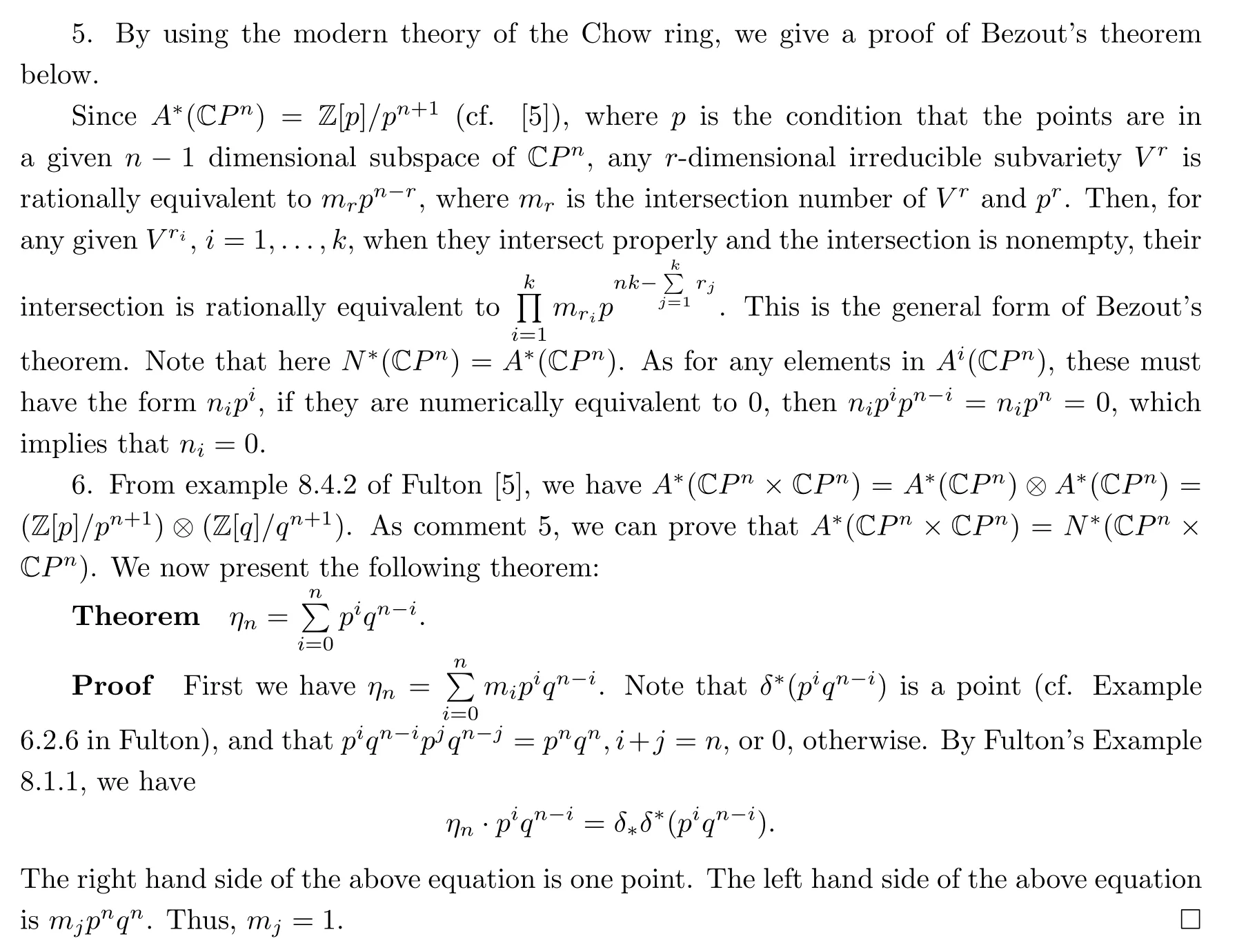
4. Schubert said the general form of Bezout’s theorem can be proved by his method.Note that Schubert only gave the proof of this theorem for three variables. To prove Bezout’s theorem for three variables, Schubert used a formula regarding η3. To get the formula for η3,he utilized a lot of formulas in B3, so to generalize his method for proving Bezout’s theorem for any n variables, similar formulas in Bnare needed. These formulas must involve elements in N∗(G(n,1)). This will be very complicated, as it seems that there is no way to get ηn+1from ηnby induction. Essentially, we feel that his method cannot be generalized to prove Bezout’s theorem for any dimensions.
4 Applications
Schubert gave six applications in §14 of coincidence formulas. The first application gives a second method for finding the number of curves in a one-dimensional system of planar curves that are tangent to a given curve in the same plane. In §4, Schubert had already obtained the number by the application of the principle of the conservation of numbers. We have already given a rigorous proof for Schubert’s first ‘proof’[3], where the application of nonstandard analysis is essential. For the rigorous description of one-dimensional system there, however,nonstandard analysis is not essential. We first give a rigorous description of matters in the framework of standard analysis.
A system of planar curves must first have the same degree, say r > 1. Its element can be represented by parameters in CPR, where R=r(r+3)/2,and this system is a variety of CPR.All the points in CPRwhich represent irreducible curves of degree r in CP2form a Zariski open set. For simplicity, we should assume that this variety representing the system is irreducible,and is denoted by Σ. Otherwise, each component of this variety can be considered separately.
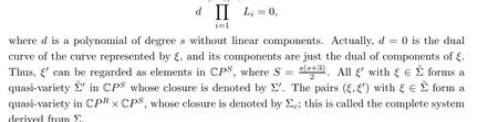
Now we give the definition of dual curves. For an irreducible curve in CP2, with the exception of singular points on the curve, there is a unique tangent line of the curve passing through the point. These tangent lines form a one-dimensional quasi-variety in CP2, and is regarded as a space of lines. The closure of this quasi-variety is an irreducible curve which is just the so called dual curve in the literature. We call the degree of the dual curve the ‘rank’of the curve, following Schubert, though it is usually called the ‘class’ of the curve (for example,Van der Wareden[6], Griffiths and Harris[7]). Schubert, however,used the word‘class’ for the degree of the dual surface. For a nonsingular curve with degree r, the rank is r(r-1), but for an irreducible singular curve with degree r, the rank must be less than r(r-1). Let [z0,z1,z2]be the coordinate of the dual plane. We denote the dual curve by d(z0,z1,z2)=0.
For a reduced curve f =0,let f =f(1)···f(s)f(s+1)···f(s+t)=0 be its irreducible decomposition,where f(1),...,f(s)are of a degree greater than one,and others are of degree one. The dual curves of the s components f(1)=0,...,f(s)=0 are d1(z0,z1,z2)=0,...,ds(z0,z1,z2)=0. For line components, there is no dual curve, so we let ds+1,...,ds+tbe nonzero polynomials of degree zero. The dual curve of f = 0 is defined to be d = d1···ds+t= 0. We define the degree of d to be the rank of the curve f =0. Thus if all the components are lines, the rank is zero.
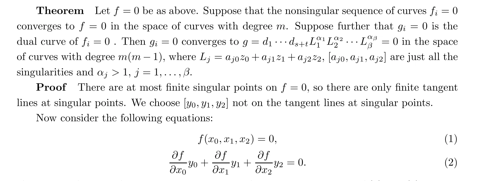
If the curve f =0 is of rank n, then the number of nonsingular solutions of (1)and(2)are just n. Thus the line y0z0+y1z1+y2z2=0 intersects the dual curve d=0 with n points. Note that[aj0,aj1,aj2]are singularities of f =0,so they are solutions of(1),(2)with multiplicity αj>1,j =1,...,β. Then, the line y0z0+y1z1+y2z2=0 intersects the line aj0z0+aj1z1+aj2z2=0 with multiplicity αj, j =1,...,β.
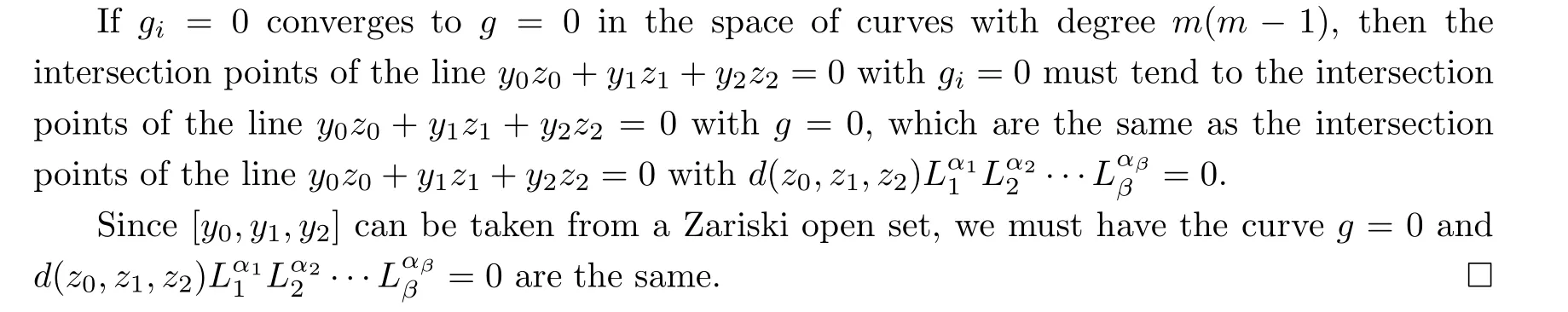
Let (1i), (2i) be the equations obtained by replacing f by fiin (1) and (2). According to the continuity of solutions with respect to coefficients, the solutions in (1i),(2i) must tend to the solutions to (1),(2). Among these, there are n solutions that tend to n points on f = 0 which are not singular points and the tangents at these are not passing through [y0,y1,y2]. In other words,there are n intersection points of the line y0z0+y1z1+y2z2=0 with gi=0 in the dual plane tending to the intersection points of the line with the dual curve d=0. Then there are αjsolutions of (1i),(2i) tending to [aj0,aj1,aj2]; that is, there are αjintersection points of the line y0z0+y1z1+y2z2= 0 with gi= 0 tending to the intersection points of the line y0z0+y1z1+y2z2=0 with (aj0z0+aj1z1+aj2z2)αj=0.

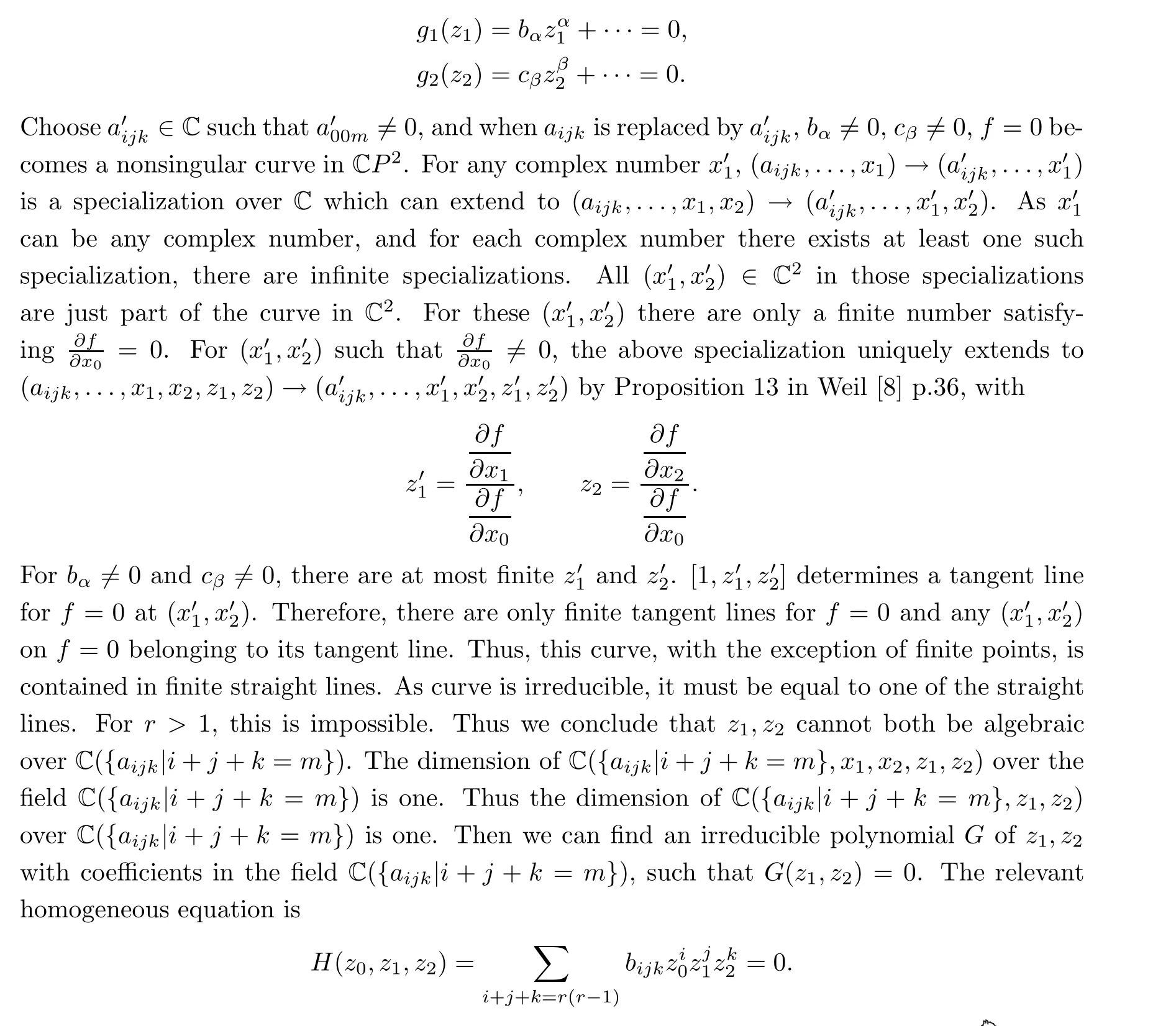
Assume that neither z1,z2are independent over C({aijk|i+j+k = m}). Then there are two algebraic equations about z1and z2with coefficients in C[{aijk|i+j+k =m}] such that
The specialization of[...,bijk,...]over C forms a subvariety in CPD. The specialization of the pair ([...,aijk,...],[...,bijk,...]]) over C forms a subvariety Crof CPR×CPD. We call Crthe set of complete curves with degree r such that if(ξ,ξ')∈Crand the curve represented by ξ has no multiple components, then ξ'is uniquely defined. Moreover,as the dual of a dual curve is the original curve, the map ξξ'is a birational equivalence. The image of this birational map is denoted by Dr.
Now we recall the definitions of systems. We have defined a one-dimensional system in [3],and any-dimensional systems in [1]. We have assumed that for a nonempty Zariski open set of the system, the curves are irreducible and the dual curves have the same rank n. That the assumption of the same degree implies the same rank is proved here.
In the space of curves with degree r(r-1), for each i, 1 ≤i ≤r(r-1), all the curves of the form
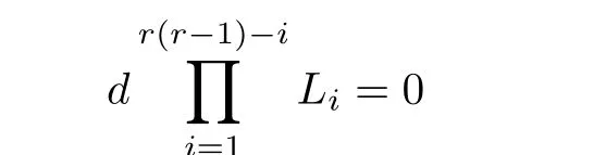
and in Drform a subvariety Riwhere d is a polynomial of degree i. We have

where Rr(r-1)is just the space of curves with degree r(r-1).
Letting Σ be an irreducible variety in CPR, there is a nonempty Zariski open set in Σ such that the elements in this set represent irreducible curves. The map ξξ'is well defined on this open set. There exists a minimum s such that Rscontains the whole image of the open set. As the curves have no linear components, n must be greater than 1. Rs-1is a closed subset of Rs. Thus RsRs-1is a nonempty open subset in Rs. The image of the open set is a quasi-variety. The inverse image of the intersection of this quasi-variety and RsRs-1is a Zariski open set in Σ, denoted by ˜Σ. The image of ξ in ˜Σ can be uniquely represented by the form
Recall that in [1], we considered the system of planar curves in space. The set of all planar curves of degree r in CP3is a CPRbundle over CP3∗. In [1], we assumed, following Schubert,that for a nonempty Zariski open set of the system,the dual curves have the same rank n. Using the same method as above, let Σ be an irreducible variety in a CPRbundle over CP3∗and there is a nonempty Zariski open set in Σ such that elements in this set represent irreducible curves. The map ξξ'is also well defined. We can also extend the definition of sets Rito the subsets of the bundles and find the minimum s such that Rscontains the whole image of the Zariski open set. Then the rank of the curves in the system is actually determined by Σ.As above, we can define the set ˜Σ and ˜Σ'and Σcas the closure of the graph of the birational correspondence between ˜Σ and ˜Σ'. We use Σcto denote the complete system determined by Σ and also by Σ'. Notice that in [1], the notation Σ was used to represent the complete system,but here Σ is only a variety in the bundle CPRover CP3∗.
We return to the first application of Schubert in§14. Schubert proved his formula as follows:
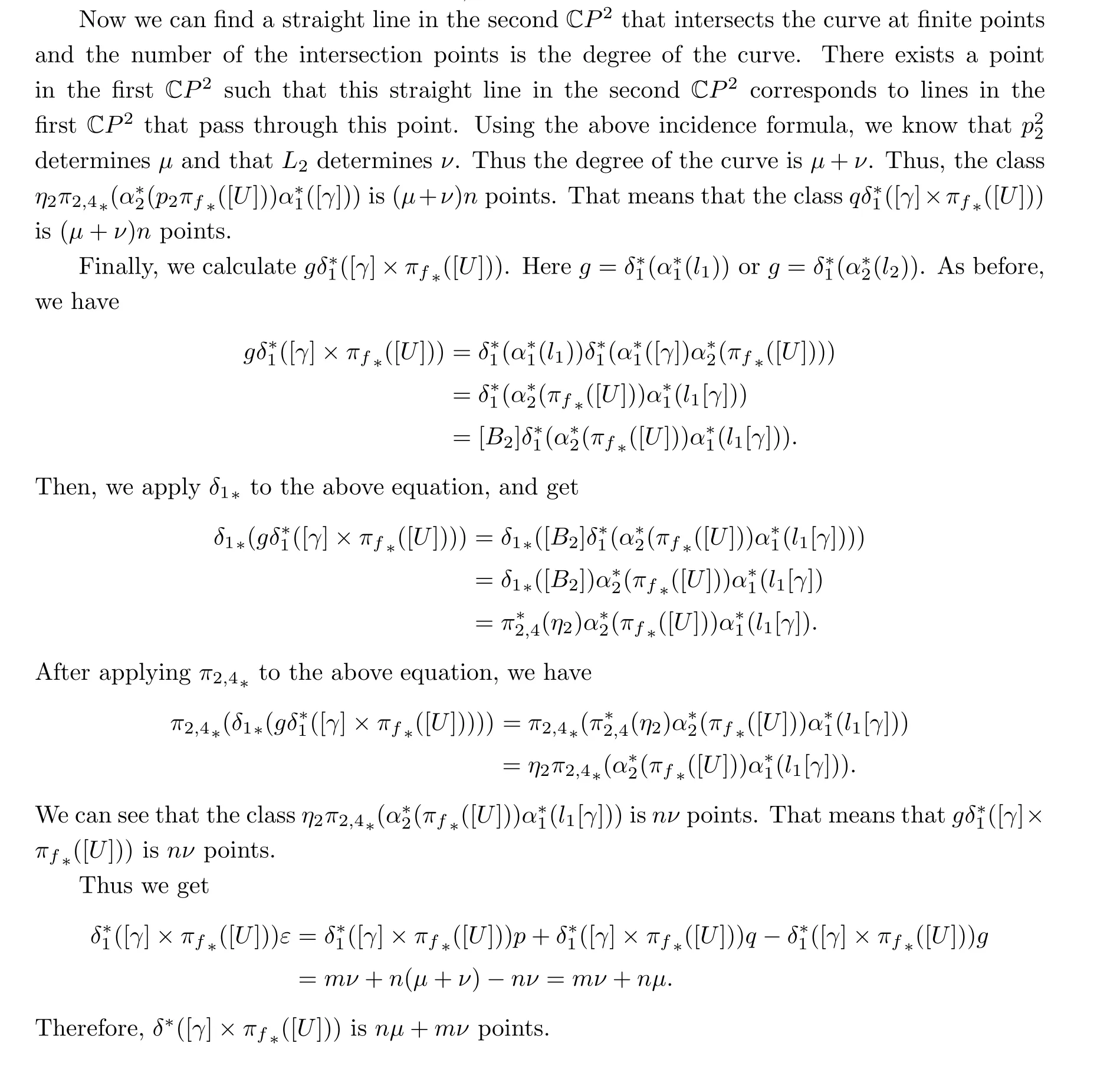
“For each tangent line g of the planar curve, the tangent point p at the planar curve and the point q such that g is tangent to a curve in the system at point q form a pair of points. Such pairs of points constitute a one-dimensional system of paired points. We apply the formula for one-dimensional systems of pairs of points

to this system. Here, p is replaced by mν, where m is the degree of the planar curve and ν is the number of curves in the system that are tangent to a given line. This is because the plane determined by p intersects with the planar curve at m points, and each tangent line at these m points are tangent to ν curves in the system. For q, note that the plane determined by q intersects with ∞1curves in the system. Thus, there are ∞1intersection points. The tangents lines at these points constitute a one-dimensional system of lines,whose degree can be obtained by incidence formula I)in§7, that is, µ+ν,where µ is the number of curves in the system that pass a given point. On the other hand, if the given planar curve is of rank n, all of its tangent lines constitute a curve of degree n in the space of lines. Then, according to Bezout’s theorem,these two curves of lines have (µ+ν)n common lines. So q is replaced by (µ+ν)n. For g, we draw n tangent lines of the planar curve at the intersection point between the line determined by the condition g and the plane where the planar curve lies. Then, we get the pairs of points on these tangent lines, where one is the tangent point at the planar curve and the other is the tangent point at some curve in the system. Thus, g is equal to nν. Therefore, we get
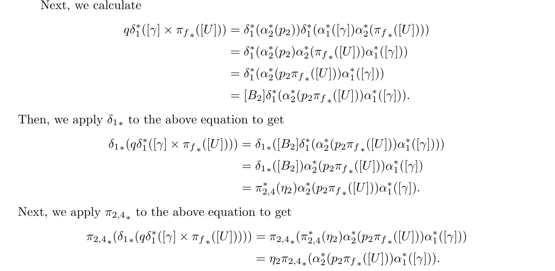
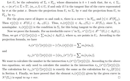
Now we give the rigorous proof of this, following Schubert’s ideas. Here Σcis a one dimensional system of planar curves as in the above discussion. Let U be a subvariety of Σc×CP2×CP2(the second CP2is regarded as the space of lines)whose dimension is dim Σc+1 such that for σc∈Σc, σc=(σ,σ')∈˜Σ× ˜Σ', (σc,x,l)∈U if and only if l is the tangent line of the curve represented by σ at the point x.
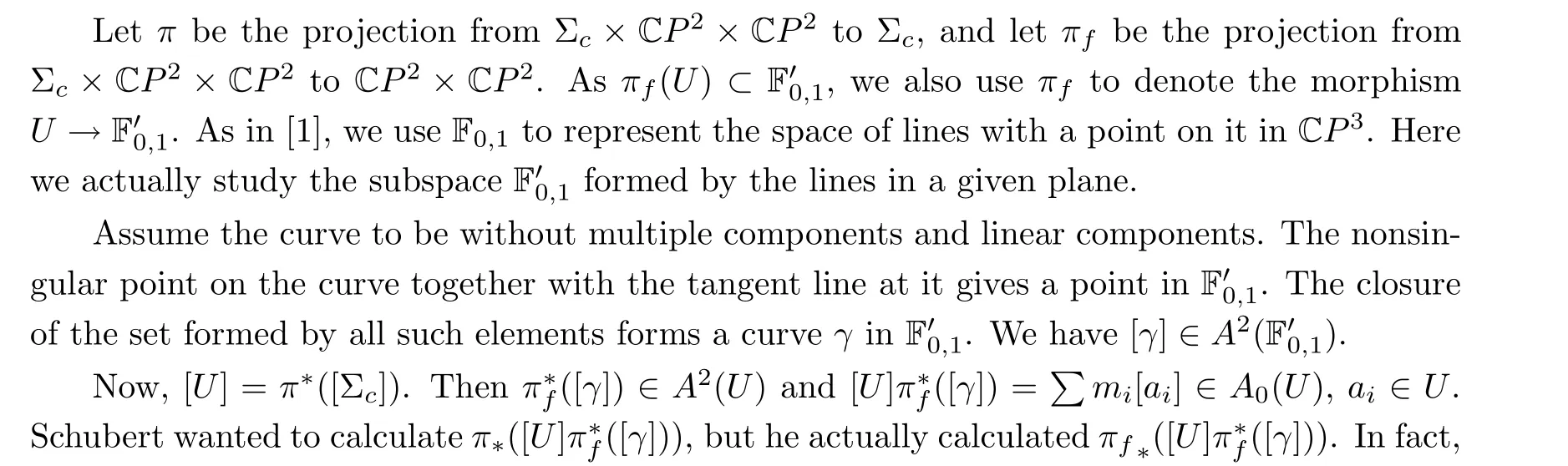
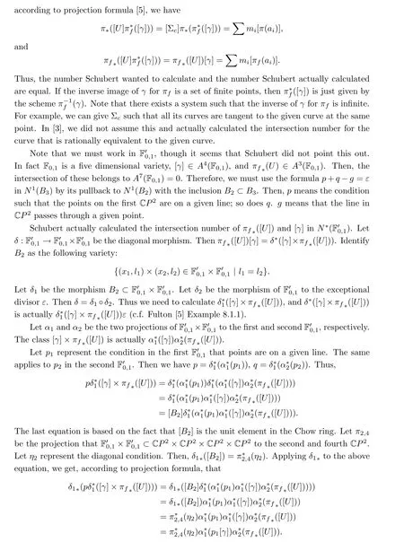
Applying π2,4∗to the above equation, we get

If α2(πf(U)) is one-dimensional, there are only finite irreducible components of this curve.However,different elements in ˜Σ'represent different curves in the second CP2. Thus the image of these under α2◦πfcannot be contained in these finite curves. Then, α2◦πfis surjective,and so is α1◦πf. Thus, except for finite points, the number of the inverse images under α2◦πfis finite (that is, ν). Thus there are only finite tangent lines of the given curve, as points in the second CP2have infinite inverse images under α2◦πf. Thus, there are only finite points on the curve with a tangent line in the above set of lines, and we can take a line to intersect with the curve at m points which are all not among the exception points just mentioned. At each of the m points, the tangent lines are just tangent to ν curves in the system. That means that the class η2π2,4∗(α∗1(p1[γ])α∗2(πf∗([U]))) is mν points. Thus, the class pδ∗1([γ]×πf∗([U]))is mν points.
As α1◦πfis surjective, there are at most finite points whose inverse image under α1◦πfis infinite. We choose a line in CP2that does not pass through these finite points. For each point on this chosen line, there are µ curves in Σ passing through this point. For any σ ∈Σ ˜Σ, the tangent line of σ at the intersection point of σ with the chosen line regarded as a point in the second CP2belongs to the union of all the σ'∈Σ' ˜Σ'regarded as subsets of the second CP2.Thus, all the tangent lines of the elements of Σ with tangent points on the chosen line form a curve in the second CP2.
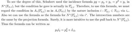
where p2represents the condition such that points are on a given line,l2represents the condition that lines pass through a given point, and L2represents the condition that the set of lines is formed by a given line on the second F'0,1.
5 nµ+mν as a Condition
In the above section, we calculated the number of curves in a one dimensional system that are tangent to a given curve of degree m and rank n, so a natural question is: can this curve define a condition in any system of planar curves? For example,in§37 Schubert gave a condition z on a system of planar conics that are tangent to a curve of degree 3 and rank 4. He did not,however, prove this according to our rigorous meaning. In a general case, Σcmay be singular.It seems to be difficult to answer the problem for general Σc. So far we only see that Chasles and Schubert have claimed that it is a condition for systems of complete conics in a plane and the given curve is either a conic or a curve of degree 3 and rank 4. Thus we have the following
TheoremLet Σcbe a system of dimension k which is a nonsingular variety. µ and ν can be regarded as elements in N1(Σc). Any curve of degree m and rank n without multiple components and linear components defines an element in N1(Σc) which is equal to nµ+mν.
ProofAs curves passing through a given point are in N1(CPR), the pull back of this under the inclusion Σ ⊂CPR, and further under the projection from Σcto ˜Σ, is in N1(Σc).This isµ. For a curve that is tangent to a given line, this is equivalent to its dual curve passing through a given point, which gives an element in N1(CPS). The pull back of this element by the inclusion ˜Σ'⊂CPSand, further, by the projection from Σcto ˜Σ', is in N1(Σc). This is ν.
AcknowledgementsThis work was partially supported by National Center for Mathematics and Interdisciplinary Sciences, CAS.
 Acta Mathematica Scientia(English Series)2022年2期
- Acta Mathematica Scientia(English Series)的其它文章
- ARBITRARILY SMALL NODAL SOLUTIONS FOR PARAMETRIC ROBIN (p,q)-EQUATIONS PLUS AN INDEFINITE POTENTIAL∗
- SUP-ADDITIVE METRIC PRESSURE OF DIFFEOMORPHISMS*
- SHARP DISTORTION THEOREMS FOR A CLASSOF BIHOLOMORPHIC MAPPINGS IN SEVERAL COMPLEX VARIABLES*
- ON CONTINUATION CRITERIA FOR THE FULLCOMPRESSIBLE NAVIER-STOKES EQUATIONS IN LORENTZ SPACES*
- ON (a ,3)-METRICS OF CONSTANT FLAG CURVATURE*
- A NOTE ON MEASURE-THEORETICEQUICONTINUITY AND RIGIDITY*