Numerical study of viscosity and heat flux role in heavy species dynamics in Hall thruster discharge

Andrey SHASHKOV,Alexander LOVTSOV,Dmitri TOMILIN and Dmitrii KRAVCHENKO

JSC ‘Keldysh Research Center’,8 Onezhskaya st.,Moscow 125438,Russia

Abstract A two- and three-dimensional velocity space axisymmetric hybrid-PIC model of Hall thruster discharge called Hybrid2D has been developed.The particle-in-cell(PIC)method was used for neutrals and ions(heavy species),and fluid dynamics on a magnetic field-aligned(MFA)mesh was used for electrons.A time-saving method for heavy species moment interpolation on a MFA mesh was developed.The method comprises using regular rectangle and irregular triangle meshes,connected to each other on a pre-processing stage.The electron fluid model takes into account neither inertia terms nor viscous terms and includes an electron temperature equation with a heat flux term.The developed model was used to calculate all heavy species moments up to the third one in a stationary case.The analysis of the viscosity and the heat flux impact on the force and energy balance has shown that for the calculated geometry of the Hall thruster,the viscosity and the heat flux terms have the same magnitude as the other terms and could not be omitted.Also,it was shown that the heat flux is not proportional to the temperature gradient and,consequently,the highest moments should be calculated to close the neutral fluid equation system.At the same time,ions can only be modeled as a cold non-viscous fluid when the sole aim of modeling is the calculation of the operating parameters or distribution of the local parameters along the centerline of the discharge channel.This is because the magnitude of the viscosity and the temperature gradient terms are negligible at the centerline.However,when a simulation’s focus is either on the radial divergence of the plume or on magnetic pole erosion,three components of the ion temperature should be taken into consideration.The non-diagonal terms of ion pressure tensor have a lower impact than the diagonal terms.According to the study,a zero heat flux condition could be used to close the ion equation system in calculated geometry.

Keywords:Hall thruster,hybrid-PIC model,moments of distribution function,magnetic-fieldaligned mesh

1.Introduction

The development of Hall thruster(HT)discharge computational methods brings us closer to understandingE×Bdischarge physics.The developed calculation models could be divided into groups according to several criteria.The first criterion is the number of dimensions of modeling.The models could be one-dimensional(1D)(axial(Z)[1–9],radial(R)[10,11]and azimuthal(θ)[12–15]),two-dimensional(2D)(Z–Rplane[16–33],Z–θ plane[34–38]),or threedimensional(3D)[39,40].On one hand,1D models do not correctly take into account the essential curvature of the magnetic field lines and plasma–wall interaction.On the other hand,3D models are too computationally expensive and existing methods used to speed-up the calculation bring about essential distortion of calculation results.For this reason,2Dmodels are the most relevant for engineering applications.The second criterion is the method of modeling plasma components.There are three methods:kinetic[12–15,27–40](direct kinetic(DK)[41]and particle-in-cell[42,43]),fluid[5,7,10,11,19,22–25]and hybrid[1–4,6,8,9,16–18,20,21](commonly with fluid electrons and kinetic neutrals and ions).Each method has pros and cons partially described in[22,41,44]and illustrated in table 1.

The kinetic method implies finding the distribution function(DF)from the Boltzmann equation using the Poisson equation.In this case,the equation system is closed;however,it demands large computational time to solve.The fluid method allows substantially reducing computational time and obtaining a smooth solution without numerical distortion of time and dimensional scales due to solving the equation systems on moments of DF instead of DF itself.Unfortunately,that brings the scientific community to the problem of closing an endless chain of equations on DF moments.

The most widespread closing method for equation systems on moments in Hall thruster modeling is using the Fourier assumption,with the heat flow(third moments)dependent on the temperature gradient(second moments)and zero non-diagonal terms of the pressure tensor(second moments).However,the correctness of the Fourier assumption in Hall thruster discharge should be proven before using it in plasma modeling.

In this work,all terms of the pressure tensor and heat flux of ions and neutrals were calculated using the developed 2D hybrid-PIC model to study the applicability of the Fourier assumption in fluid models.Section 2 offers some information about the way the authors define the DF moments and the suggested method of studying the moments’ impact on heavy species dynamics.In section 3,the 2D hybrid-PIC model is described.Results and discussions are provided in section 4.Finally,section 5 reports the conclusion of the work.

2.Moments of distribution function

3.Numerical model

The developed numerical model is called Hybrid2D,which implies use of the PIC method for heavy species and the fluid method on aB-field aligned mesh for electrons.The nearest analogs for Hybrid2D are the hybrid-PIC model HPHall-2[20]and the fluid model Hall2De[22].The electron fluid submodel of Hybrid2D is analogous to Hall2De and differs from HPHall-2 in its absence of the thermalized potential assumption[45]and MFA mesh near the walls.The heavy species submodel of Hybrid2D differs from Hall2De in that it comprises fully kinetic ions and boundary conditions on the cathode.As opposed to Hybrid2D,the latest version of Hall2De comprises the emitting surface method for neutrals and a hybrid-PIC model for ions,with slow ions modeled as a cold non-viscous fluid and fast ions modeled with the PIC method[46].The cathode boundary in Hall2De is modeled using the data from the independent ORCA2D cathode fluid model[47].

3.1.Simulation region

The scheme of the simulation region is shown in figure 1.The simulation region is a dotted region,which includes a discharge chamber and the nearest plume region.The discharge chamber of the modeled thruster has conducting walls and insulating rings at the exit.Magnetic poles are covered with Al2O3,which is also an insulating material.The symmetry axis is out of the simulation region.Therefore,the down boundary is a free boundary.The cathode boundary is shown as a bold solid line in figure 1.The boundary is placed between two magnetic field lines,which cross the lower and the upper edges of the cathode,placed outside of the simulation region.The model is axisymmetric.It seems incorrect to model the cathode boundary directly at the cathode diaphragm location,where the flow of primary electrons is still localized in the azimuthal direction.Assuming that the primary electrons move from the cathode to the plume mainly along the magnetic field lines under the action of the pressure gradient and in the azimuth direction under the impact of the E×B drift,the cathode boundary can be located at the edge of the simulation region,as shown in the figure.All walls in this study have a temperature of 600 K.The magnetic field is exported from Magnet2D[48].

3.2.Computational mesh

The PIC method commonly implies using a regular rectangle mesh.In this case,localization of a particle on the mesh is done through simple integer division,which is extremely important to minimize the computational cost.In the case of the MFA mesh,the localization of the particle is less obvious.In HPHall-2,to localize the particles,the MFA mesh was transformed to a regular one with the Jacobian calculated in a pre-process stage.Such a method cannot give a strongly aligned mesh in all simulation regions and leads to numerical diffusion.In Hybrid2D,we use three meshes(see figure 2)connected in a pre-process stage for particle localization.The rectangular mesh shown in figure 2(a)is used for preliminary localization of the particles in the simulation region.The MFA mesh shown in figure 2(b)is used to solve the fluid equation system.The triangular mesh shown in figure 2(c)is used for detailed localization of the particles on the MFA mesh and interpolation of the particle moments to the centers of the MFA mesh.

The connection between the meshes is illustrated in figure 3.The rectangular mesh is a basic mesh,which covers the entire simulation region uniformly.The MFA mesh is constructed above the regular one using the exponential compression technique[49,50].The triangular mesh is constructed in such a way that the vertices of triangular cells are placed at the centers of MFA cells.In the pre-processing stage,each rectangular cellRrefers to the list of all triangular cells that cross the square of theRcell.In the processing stage,the localization of the particlePhas two stages:(1)localization of particlePat the rectangular mesh by simple integer division,(2)particlePis found to be inside of one of the triangles referred to asRcell in the pre-processing stage.The particle is inside a triangular cell when the half-line with the start inPemitted in a random direction crosses the cell edges of that triangular cell once.After the particle is localized,the particle is weighed at triangular cell vertices,which at the same time are the nodes of the MFA mesh.The correcting volumes were used for weighting to take into account the axisymmetric geometry of the simulation region[51].

3.3.Electron fluid submodel

PIC submodel yields the moments of neutrals and ion in the centers of MFA cells.Assuming quasi-neutrality and single ion charges only(multiple-charged ions at this stage were not taken into account,but consideration of them does not change the logic of the paper),electron concentration could be found from the ion concentration:

whereni,ne,andnare ion,electron and plasma concentrations,respectively.Continuity equations for ions and electrons yield

where the total,electron and ion current densities are given byj=je+ji,je= −enue,andji=enui,respectively,andueanduiare the electron and ion fluid velocities,respectively.

Assuming zero electron inertia and viscosity terms,electron momentum conservation is given by

where the total momentum transfer frequency is

The electron equation system was solved in terms of projections on the MFA mesh.Directions along and across the magnetic field lines are noted as χ andψ,respectively.According to these notations,projections of electron momentum equation on MFA coordinates are given as

where electron mobility is given as

Assuming zero electron inertia,energy conservation(4)could be written as

whereκ is the heat conductivity defined as

In MFA projections,the electron heat flow is given as

The linear dependence of the heat flow on the temperature gradient is obtained by neglecting the electron fluid motion.It seems inconsistent to neglect the electron motion in equation(21)and not neglect it in equation(20).However,this approach was used in[22]and gives good agreement between the modeling results and the results of the experimentally measured ion velocity distribution in the discharge channel.Although the closing method(21)should be verified more accurately in the future,such examination is outside the scope of this work.

3.4.Boltzmann integrals

Using relaxation assumption and assuming collisional anomalous conductivity model,Boltzmann integrals could be found as

where the following notions were made:

whereνi,νex,νen,νei_clmb,νaare the single electron–neutral ionization,electron–neutral excitation,elastic electron–neutral collisions,electron–ion Coulomb collisions,and electron anomalous collision frequency,respectively;γiandγexare the ionization and excitation losses,respectively;∊0is the vacuum permittivity.

Electron anomalous conductivity was defined as it was proposed in[53]:ωCL(z,rCL)is the electron cyclotron frequency at the cen-

wherezandrare the axial and radial directions,respectively,terline in the point,which is contained in the magnetic line,crossing the point(z,r),a(z)is the conductivity coefficient:

wherefjare the conductivity coefficients,defined at semiopen intervalz∊[zj−1,zj).The coefficientsfjtake on values from 0 to 1,indicesjtake on integer values from 1 to 6.In the case wherez>z6,the conductivity coefficient becomes constanta=f6.The coefficientszjandfjwere calculated in the 1D3V hybrid model[9,54]using the adjustment of the anomalous conductivity profile to experimentally measure the operating parameters described in detail in[55].Figure 4 shows the anomalous collision frequency profile in comparison with classical collision frequencies and the electron cyclotron frequency.Table 2 shows the adjusted values of the coefficientszjandfj.

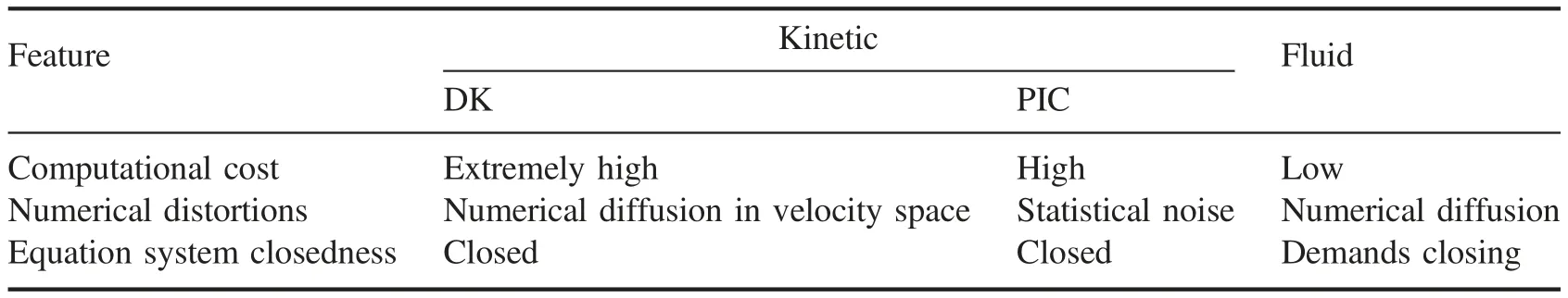
Table 1.Features of various modeling approaches.

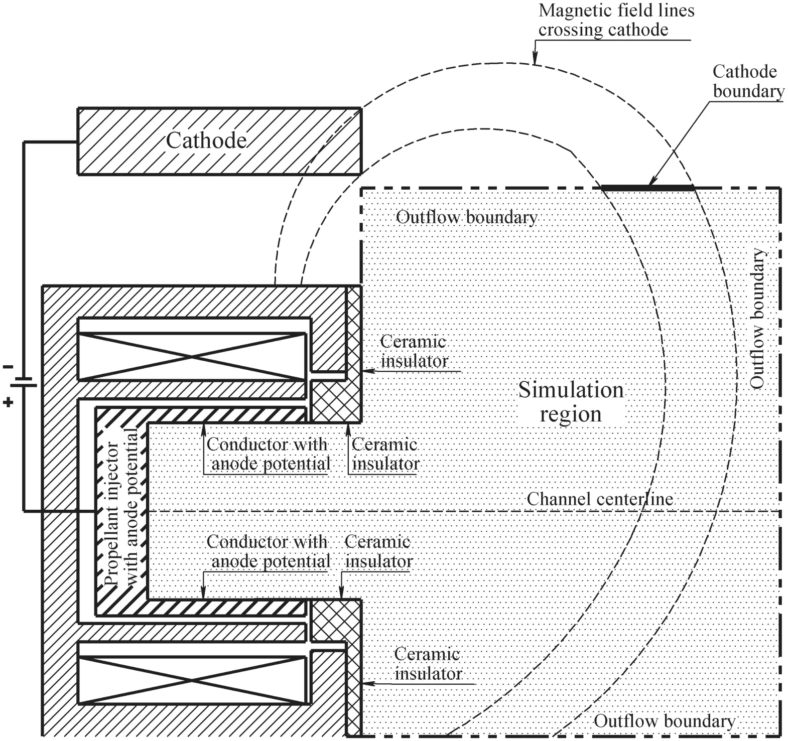
Figure 1.Scheme of the simulation region.

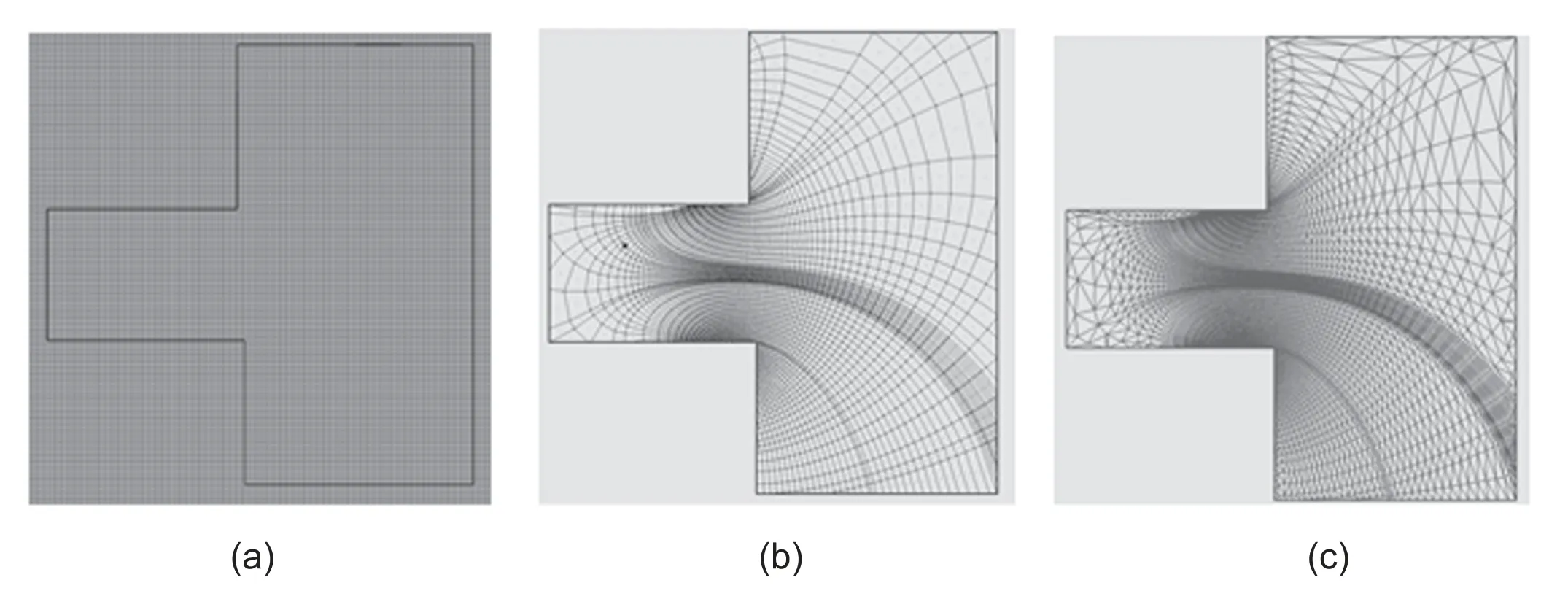
Figure 2.Types of meshes used in Hybrid2D:(a)structured regular orthogonal rectangular mesh(rectangular mesh),(b)structured irregular orthogonal magnetic field-aligned mesh(MFA mesh),and(c)structured irregular non-orthogonal triangular mesh(triangular mesh).

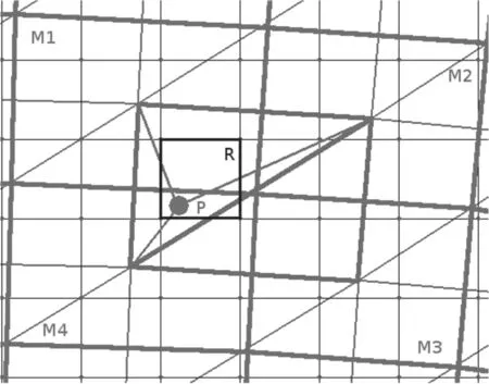
Figure 3.Particle weighting using Hybrid2D meshes.

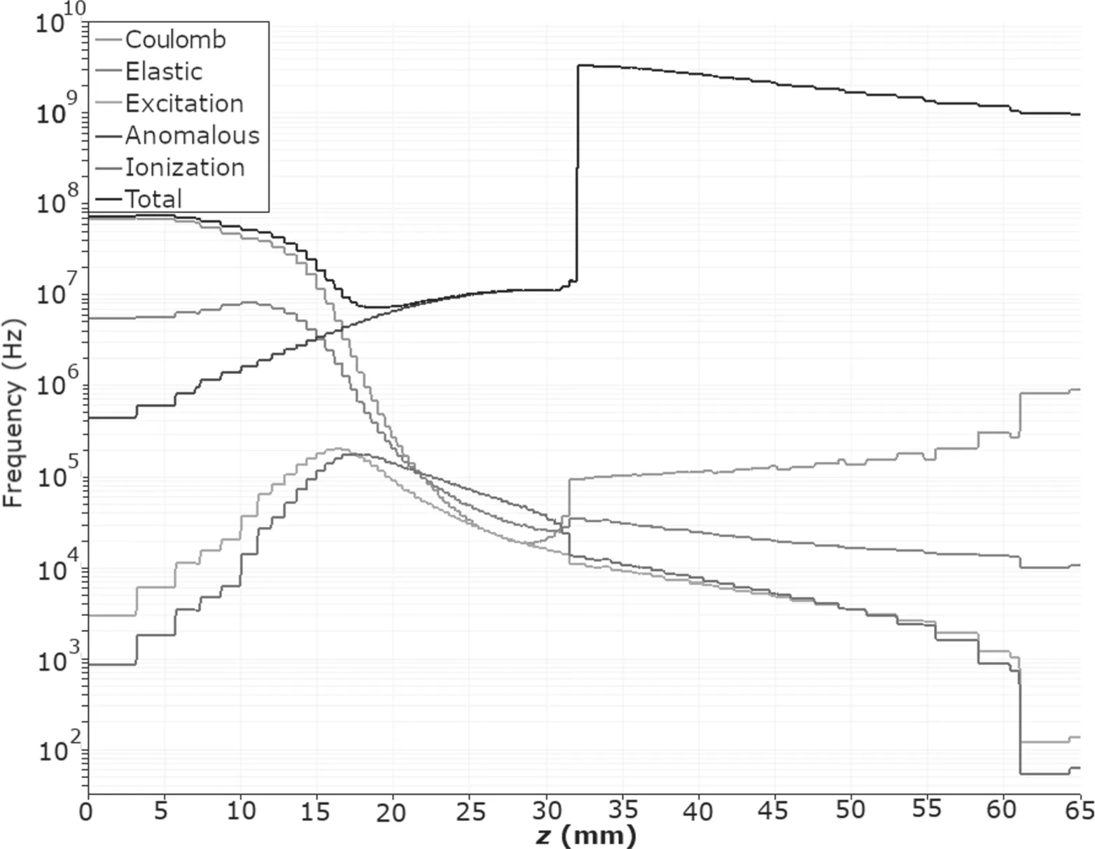
Figure 4.Anomalous collision frequency in comparison with classical collision frequencies.

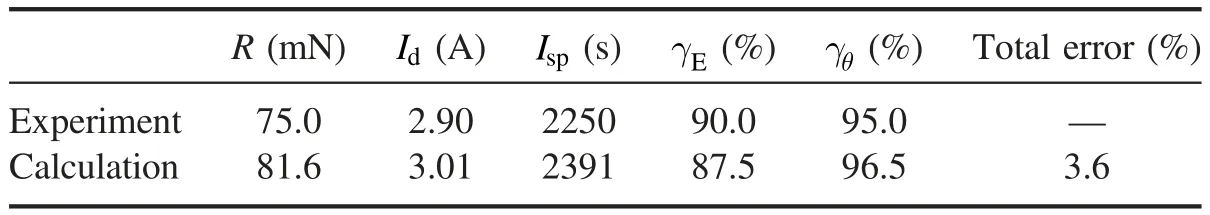
Table 3.The operating parameters of the KM-88 in calculation and in the experiment.

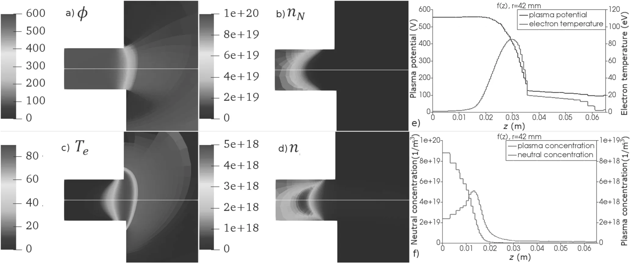
Figure 5.Plasma parameters and first moments.On the r–z plane:(a)plasma potential,(b)neutral concentration,(c)electron temperature,(d)ion concentration.Along the centerline:(e)plasma potential and electron temperature,(f)neutral and ion concentrations.

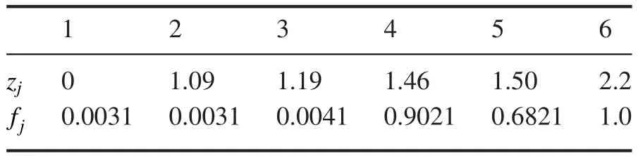
Table 2.The anomalous collision profile coefficients,adjusted in the 1D3V model in accordance with the experimentally measured operating parameters.

3.5.Boundary conditions

There are four types of boundary conditions in the model:anode,cathode,ceramics and free boundary.The neutrals are reflected diffusively with the wall temperature by the anode and ceramics.The cathode and free boundary are transparent for neutrals and ions.The ions recombine at the anode and ceramics.As a result of ion-wall recombination,neutrals are reflected from the wall diffusively.

The boundary condition for ion velocity at the wall requires special attention.On one hand,the ion velocity at the walls should meet the Bohm criterion.On the other hand,theion velocity at the boundaries is defined by the PIC submodel and cannot be corrected in accordance with the Bohm criterion directly.Meeting the Bohm criterion could be the problem in hybrid simulations.However,in calculations carried out in this work,in a quasi-steady solution,the PIC flow of the ions to the walls automatically meets the Bohm criterion.

The electron boundary conditions are described below.Indexccorresponds to the cell center number,and indexbis the edge of the cellcallied with the border.

Assuming the heat velocity for the electrons in the presheathaccording to the Boltzmann distribution,the electron flow to the walls is defined as

The potential drop at the ceramics is defined with the assumption of the secondary electron emission and the wall charge balance[56]:

wheremiis the ion mass,σSEEis the secondary electron emission coefficient,equal to zero for the anode and given by[57]for the ceramics:

The potential drop at the free boundary is equal to zero:

The potential drop at the anode depends on the potential at the near boundary cell(34),which,in turn,depends on electron current density at the anode(33),depending on the potential drop.The problem is self-consistent and should be solved implicitly[22]:

The electron current density in ceramics and the free boundary is defined by the charge balance condition:

The conductive heat flux to the boundaries is set to zero,The electrons convective heat flux to the boundaries is given by

At the cathode boundary,the plasma potential and the electron temperature are set to 0 V and 1.5 eV respectively.The plasma concentration gradient at the cathode boundary is set to zero.In this case,the electron current density from the cathode is determined by the electron momentum equation projections(17)and(18).

3.6.Numerical scheme

The finite volume method with the first-order approximation was used to solve the electron equation system.Incidentally,the electron continuity equation(14)with the electron current density from equations(17)and(18)integrated in each cell over the volume using Gauss’ theorem yields:

Taking into account the boundary conditions,the plasma potential could be found implicitly as:

where the following notations were made:

where the following notations were made:

The numerical scheme in equations(43)and(51)is a five-node implicit scheme.The equation system could be written in matrix form as the equality of the product of an unknown vector and aN×Nfive-diagonal sparse matrix,whereNis a number of cells in the calculation region,to the right part vector.The solution could be found as a product of an inverse matrix and the right part vector.The inverse matrix was found using an open-source library for parallel matrix calculations on CUDA named cuSPARSE[58].To resolve the implicit anode boundary condition,the iterative method was used.Most commonly,a maximum of three iterations were enough to find the solution.The electric field in the cell center was found using the first-order matrix method for unstructured meshes[49].This electric field acts on the ions with the same coefficients as in the weighting procedure to avoid self-acceleration.

4.The results and their analysis

The thruster KM-88 with centerline 88 mm[59]and 15 mm height of the discharge channel[54]was modeled.The simulation domain was 2.5 times longer than the discharge chamber length.The operating mode with 3.48 mg s−1of the anode flow rate and 550 V of the discharge voltage,which was set during the 1000 h wear test,was used for plasma modeling.The calculation ran until the particle balance was achieved:

whereΔJis the total particle balance,are the average neutral income,neutral outcome and ion outcome,respectively.The averaging was carried out over a 0.2 ms period of calculating time.All kinetic moments presented below were averaged during this same time.The results of the modeling are presented in table 3.Figure 5 shows the distributions of the plasma parameters(such as plasma potential,electron temperature)and zero moments(such as ion and neutral concentration)on ther–zplane and along the centerline.Here and below,the white lines on the 2D figures show the direction along which the 1D distributions are built.

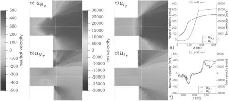
Figure 6.The first moments of neutrals and ions.On the r–z plane:(a)neutral axial velocity,(b)neutral radial velocity,(c)ion axial velocity,(d)ion radial velocity.(e)Axial neutral and ion velocity along the centerline,(f)radial neutral and ion velocity along the radius near the exit plane.

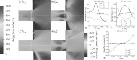
Figure 7.The second moments of neutrals.On the r–z plane:(a)component (e)Diagonal terms along the centerline,(f)diagonal terms along the radius near the exit plane,(g)non-diagonal terms along the radius near the exit plane.

Figure 6 shows the first moments of ions and neutrals.Figures 6(a)and(e)illustrate that the assumption about the constancy of the neutrals’ velocity is incorrect because,in fact,the velocity changes about five times within the discharge channel.The increase of the velocity is due to the fact that the slow neutrals take more time to cross the ionization region than the fast neutrals,which leads to the ionization of slow particles and the transit of fast particles.This effect is fully kinetic.The similarity of the neutral and ion radial velocity profiles is much less obvious to us(figure 6(f)).The magnitude of the radial velocities differs dozens of times,but their shapes are quite similar;despite this,it seems that the electric field,which affects ions and does not affect neutrals,should bring about the difference in radial velocity profiles.

Figure 7 shows neutrals’ non-zero components of the pressure tensor(second moments).The figure illustrates that the temperature in various directions has comparable magnitudes and significantly different profiles.The wall temperature in calculations was 600 K.The deviations from this value in different regions are derived from different effects.For example,the increase of the temperaturenear the ceramics(figure 7(a))is derived from the recombination of the ions collided to the wall.The velocities of the recombined neutrals differ from the velocities of primary neutrals in this region,which leads to the increase of the temperature.The decrease ofat the centerline in ionization region(figure 7(a))seems to be derived from the ionization of slow particles making the neutral flux more homogeneous.The increase ofin ionization region(figure 7(b))in our opinion is derived from the crossing of wallreflected neutrals and non-ionized direct flow from the anode.The increase oftowards the symmetry axis(figure 7(c))is likely derived from the transformation of componentto the componentwith the radius decrease.Only componentis non-zero among the non-diagonal components of the pressure tensor(figure 7(d)).

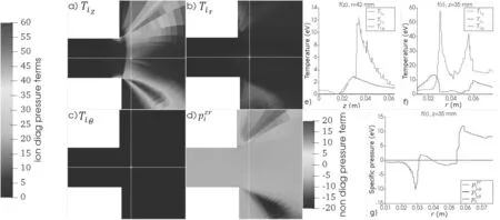
Figure 8.The second moments of ions.On the r–z plane:(a)component (e)Diagonal components along the centerline,(f)diagonal components along the radius near the exit plane,(g)non-diagonal components along the radius near the exit plane.

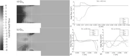
Figure 9.The third moments of neutrals.On the r–z plane:(a)axial heat flow,(b)radial heat flow.(c)Along the centerline,(d)along the radius in z = 20 mm from the anode,(e)along the radius in z=14 mm from the anode.

Figure 8 shows ions’ non-zero components of the pressure tensor(second moments).Opposed to the neutral temperature,the ion temperature in the azimuthal direction is about zero and can be neglected.IonTrcomponent is comparable withTzcomponent only in some regions(figures 8(a),(b),(e),(f)).Similar to the neutrals,only componentPzris non-zero among the non-diagonal components of the pressure tensor(figure 8(g)).The non-diagonal component is comparable with the diagonal one in the plume periphery region.

Figures 9 and 10 show the third moments for neutrals and ions,respectively.The azimuthal heat flow is near-zero for both ions and neutrals.For neutrals,the heat flows in the axial and radial directions are comparable.For ions,the axial heat flow is dominant.However,the divergence of these values should be compared with the other terms in equation(12)to determine the influence of the heat flow on the particle dynamics.

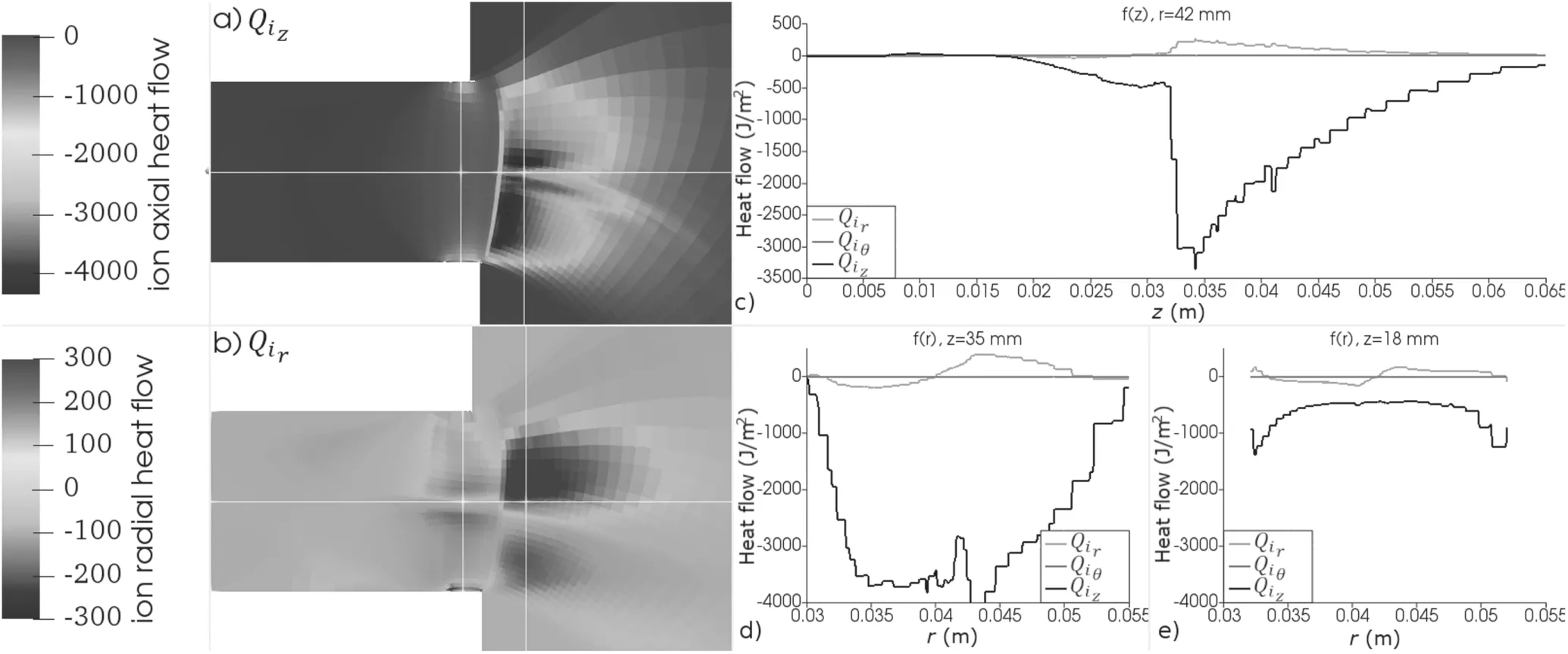
Figure 10.The third moments of ions.On the r–z plane:(a)axial heat flow,(b)radial heat flow.(c)Along the centerline,(d)along the radius in z=35 mm from the anode,(e)along the radius in z=18 mm from the anode.

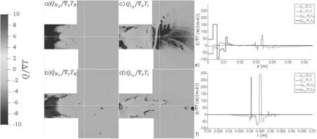
Figure 11.The ratio of the heat flow to the temperature gradient.On the r–z plane:(a)axial projection for neutrals,(b)radial projection for neutrals,(c)axial projection for ions,(d)radial projection for ions.(e)Along the centerline,(f)along the radius near the exit plane.

The Fourier assumption implies that the heat flow is proportional to the temperature gradient.Figure 11 shows absence of such a dependence,in the authors’ opinion.Consequently,in the case the heat flow significantly affects the heavy species energy balance,the next moments should be calculated to solve the closing problem.The estimation of the magnitude of the heavy species’ moments in comparison with the other terms in equations(10)–(12)is presented below.

Figures 12 and 13 show the terms in the axial(equation(10))and radial(equation(11))projections of the neutrals’ momentum.According to the calculations,the nondiagonal terms of the pressure tensor in both axial and radial projections are comparable with the diagonal ones.Figures 12(c)and 13(e)show that the non-diagonal terms partially compensate for the diagonal terms,reducing the magnitude of the convective terms.Viscosity seems counterintuitive for free molecular flow without collisions;however,neglecting the viscosity for neutrals significantly changes the force balance in the momentum equation,which leads to distortion in the neutrals’dynamics.The terms of the pressure tensor depend on the heat flow,which could be found only from the energy balance equation(12).

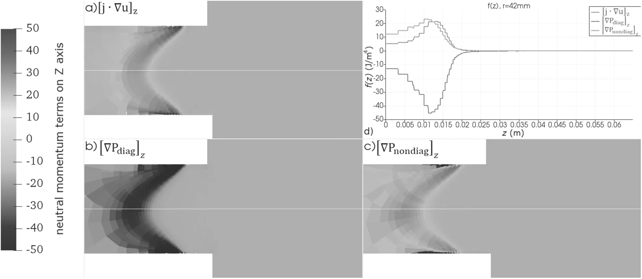
Figure 12.Axial projection of the neutrals’ momentum terms:(a)momentum convective flux,(b)gradient of the diagonal terms of the pressure tensor,(c)gradient of the non-diagonal terms of the pressure tensor,(d)terms of equation(10)along the centerline.

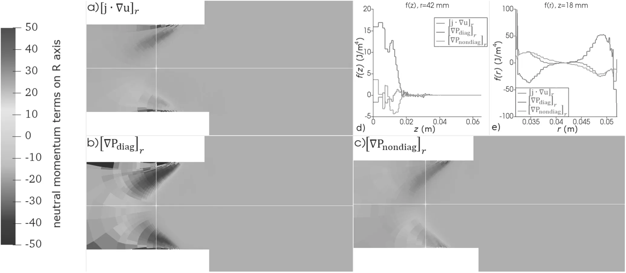
Figure 13.Radial projection of the neutrals’ momentum terms:(a)momentum convective flux,(b)gradient of the diagonal terms of the pressure tensor,(c)gradient of the non-diagonal terms of the pressure tensor(d)terms of equation(11)along the centerline(e)terms of equation(11)along the radius at 18 mm from the anode.

Figure 14 shows the terms of the neutrals’energy balance equation(12).The figure shows that the heat flux divergence and flux of the non-diagonal terms of the pressure tensor are comparable with the kinetic energy convective flux.The energy balance is provided with compensation of the convective flux of the diagonal terms of the pressure tensor by the kinetic energy convective flux,convective flux of the nondiagonal terms of the pressure tensor and the heat flow divergence.Consequently,neglecting the viscosity and heat flow terms leads to distortion of energy balance.As a result,using the first three moments is insufficient for the fluid description of the neutrals’ dynamics and correct closing is demanded.An example of the fluid model,which correctly solves the closing problem for neutrals,is shown in[60].

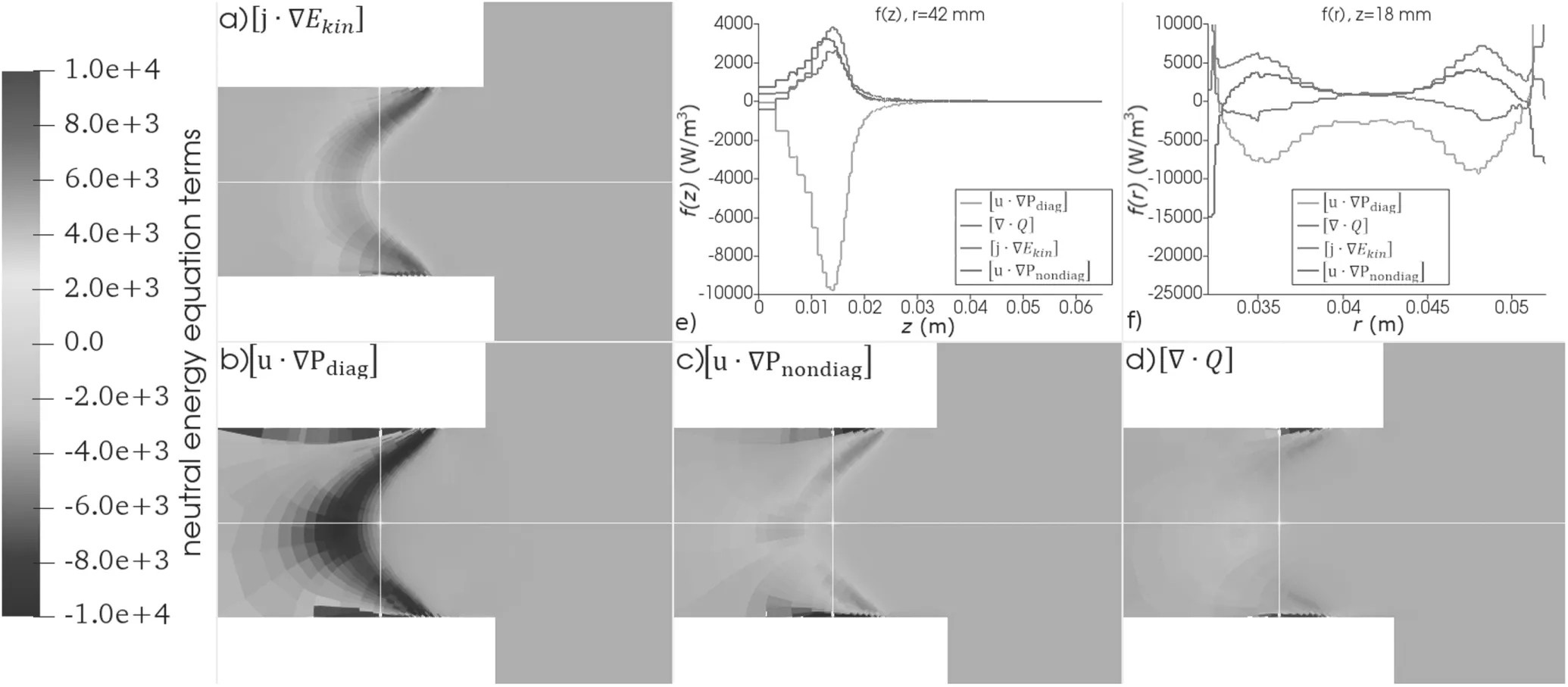
Figure 14.Terms in the neutrals’energy balance equation.On the r–z plane:(a)kinetic energy convective flux,(b)flux of the diagonal terms of the pressure tensor,(c)flux of the non-diagonal terms of the pressure tensor,(d)heat flux divergence.(e)Along the centerline,(f)along the radius at 18 mm from the anode.

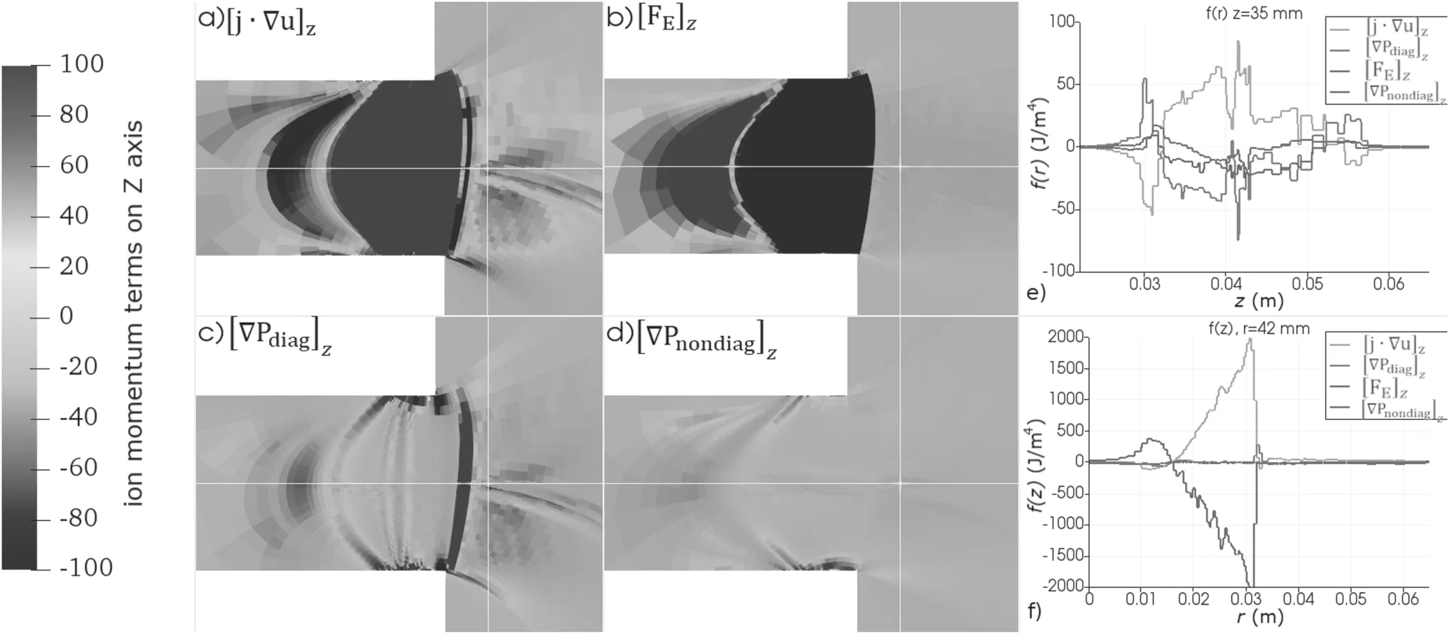
Figure 15.Axial projection of the ion momentum terms:(a)momentum convective flux,(b)electric filed,(c)gradient of the diagonal terms of the pressure tensor,(d)gradient of the non-diagonal terms of the pressure tensor,(e)terms of equation(10)along the radius at the distance of 35 mm from the anode,(f)terms of equation(10)along the centerline.

Figures 15 and 16 show the terms in the axial(equation(10))and radial(equation(11))projections of the ions’ momentum.As opposed to the neutrals,according to figure 15(f),the ion dynamics along the centerline is mostly defined by the electric field.The terms of the pressure tensor have a local impact on the ion dynamics near the exit plane at a distance of 32 mm from the anode(see figures 15(a),(c)and(f)),which leads to an insignificant ion flux slowdown(200 m s−1or 0.8% from flux velocity).However,when the operating parameters of the thruster are the focus of the study,this impact is small enough to be taken into consideration in the fluid model.Consequently,equation(10)implies no second moment terms,and a cold ion assumption could be used in fluid models,as in[22,25].However,the magnitude of the pressure tensor components becomes higher than that of the electric field terms in the plume region,where the electric field is low enough(figure 15(e)).Also,the convective terms have been compensated for by the sum of the diagonal and nondiagonal pressure tensor components at the plume periphery beside the electric field.This leads to a change in the plume divergence structure and an increase of the ion backflow to the magnetic poles.Consideration of the ions’temperature leads to the slowdown of the ion flux in the axial direction in the plume periphery region,where the maximum of the ion temperature is comparable with the electron temperature maximum according to figure 8(a),and to additional acceleration of the ion flux at the centerline.If the acceleration of the flux at the centerline is negligible in comparison to the absolute value of the ion velocity in this region,then the slowdown of the ion flux at the periphery of the plume should lead to an increase of the poles’erosion in comparison to the fluid models with cold ions.Also,the plume divergence should be increased by the ion pressure gradient,which is important to take into account to correctly place the antenna on a satellite.Figure 16 shows that the pressure tensor terms are negligible in almost all regions in the radial projection of the ion momentum equation.The only regions where the pressure tensor terms are comparable with the convective and electric field terms are the regions inside the discharge chamber near the walls and near the centerline(figures 16(c)and(e)).In these regions,the consideration of the pressure terms should lead to the acceleration of the velocity of the ion dissipation to the walls.However,the magnitude of the non-diagonal terms seems too small to affect the force balance in the radial direction at all according to figure 16.As a result,the cold ion fluid model is enough to accurately calculate the operating parameters.However,the ion temperature should be taken into account in the case where second-order effects like ion backflow to the poles and plume divergence are under study.

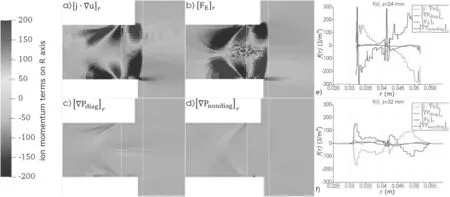
Figure 16.Radial projection of the ion momentum terms:(a)momentum convective flux,(b)electric filed,(c)gradient of the diagonal terms of the pressure tensor,(d)gradient of the non-diagonal terms of the pressure tensor,(e)terms of equation(10)along the radius at the distance of 24 mm from the anode,(f)along the radius at the distance of 32 mm from the anode.

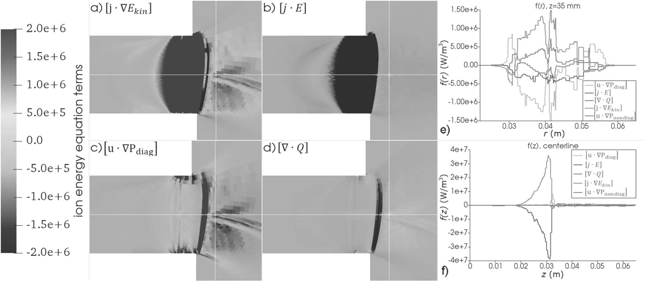
Figure 17.Terms in the ions’energy balance equation.On the r–z plane:(a)kinetic energy convective flux,(b)flux of the diagonal terms of the pressure tensor,(c)electric force work,(d)heat flux divergence.(e)Along the radius at 35 mm from the anode,(f)along the centerline.

The ion energy balance equation terms are shown in figure 17.Inside the discharge chamber,the kinetic energy flux is compensated for by the electric field work(figure 17(f)).Near the exit plane,the balance is defined by the negative kinetic energy flux and heat flux,and the positive pressure gradient(figures 17(a),(c)and(d)).In the plume region,a comparable impact of all terms of the energy balance is observed(figure 17(e)).In the plume periphery region,it is most important to define both diagonal and non-diagonal pressure tensor terms for the energy balance.According to figure 17,in this region,the heat flow and the non-diagonal terms have a lower magnitude than the diagonal terms.The minor impact allows us to close the fluid equation system using a zero heat flow assumption.Viscosity terms also have a minor impact on the energy balance and could be omitted in the energy equation.Therefore,the fluid equation system for ions should include the equations on the diagonal terms of the pressure tensor,besides equations(10)–(12),and a zero assumption for the heat flow.

5.Conclusion

A 2D hybrid-PIC numerical model of Hall thruster called Hybrid2D has been developed.The model differs from previous hybrid-PIC models by its numerical mesh,which is aligned with the magnetic field lines in the whole simulation region,including near wall regions,and by its electron fluid model,which is analogous to the Hall2De model[22].To make particle simulations on the MFA mesh more computationally affordable,the weighting method of the particles on the MFA mesh was developed.The anomalous conductivity profile for the electrons was adjusted to the experimentally measured operating parameters of the thruster using a 1D hybrid-PIC model[55].

Using the developed Hybrid2D code,the first three moments of the ions and neutrals distribution functions were calculated.The influence of the second and the third moments on the force and the energy balance was estimated.According to the results,the fluid equation system for neutrals should include more than three first moments,because each moment affects the balance significantly and the Fourier assumption is shown to be unfeasible for the neutrals in a Hall thruster.The first three moments are not enough to close the fluid equation system for neutrals.A possible method to close the neutral fluid equation system is described in[60].The fluid equation for the ions can only include the zero and the first moments when only the operating parameters of the thruster or the plasma local parameters along the centerline are under study.However,in the case that second-order effects like plume divergence or ion backflow to the magnetic poles are under study,the ion fluid equation system should also include all three diagonal terms of the pressure tensor.Fortunately,zero ion heat flow and zero viscosity assumptions could be used for the closing of the fluid equation system for ions.