
Coupled-generalized nonlinear Schr¨odinger equations solved by adaptive step-size methods in interaction picture
2023-03-13 09:19LeiChen陈磊PanLi李磐HeShanLiu刘河山JinYu余锦ChangJunKe柯常军andZiRenLuo罗子人
Chinese Physics B 2023年2期
Lei Chen(陈磊) Pan Li(李磐) He-Shan Liu(刘河山) Jin Yu(余锦)Chang-Jun Ke(柯常军) and Zi-Ren Luo(罗子人)
1Aerospace Information Research Institute,Chinese Academy of Sciences,Beijing 100094,China
2National Microgravity Laboratory,Institute of Mechanics,Chinese Academy of Sciences,Beijing 100190,China
3University of Chinese Academy of Sciences,Beijing 100049,China
Keywords: nonlinear optics, optical propagation in nonlinear media, coupled-generalized nonlinear Schr¨odinger equations(C-GNLSE),adaptive step-size methods
1.Introduction
Coupling an ultrashort laser pulses into an optical fiber,a wealth of nonlinear effects will take place due to the dispersion and the nonlinear effect of the fiber.The phenomenon has been widely used in optical fiber communication, ultrafast optical,supercontinuum generation,optical coherence tomography,etc.[1-4]The propagation of the low power ultrashort pulses in the fiber could be described by a mathematical model of the nonlinear Schr¨odinger equation (NLSE) which contains the group velocity dispersion (GVD) and self-phase modulation (SPM) terms.[2]To evaluate the high peak power femtosecond pulses, the generalized nonlinear Schr¨odinger equation (GNLSE) with the high order dispersion and nonlinear terms was adopted.[5]Although the NLSE could be analytically solved by the inverse scattering and self-similar method,[6,7]the GNLSE can only be calculated numerically.A common numerical solution to the GNLSE has been obtained by the split-step Fourier method (SSFM).[2]In the SSFM scheme, the dispersion and nonlinearity were integrated respectively in each step and the accuracy of the global error was of the second-order.[8]While the accuracy could be improved by the symmetric split-step Fourier method(S-SSFM)[9-13]or high order split-step schemes such as the fourth-order scheme of Blow and Wood,[14]the global accuracy was not better than that of the nonlinear step integration.In order to further improve the accuracy,a number of methods have been developed:A Runge-Kutta in the interaction picture(RK4IP)method was extended to solve the GNLSE and stimulate the pulse propagation and supercontinuum generation in the optic fiber by Hult.[15]The RK4IP exhibits a fifth order local accuracy and high calculation efficiency in the fixed step methods.The conservation quantity error adaptive step-control algorithm based on RK4IP(RK4IP-CQE)was introduced to solve the GNLSE by Heidt in 2009.[16]The RK4IP-CQE,an effective and accurate numerical method of GNLSE solution,reduced more than 50% computational time than the local error adaptive stepcontrol method.[17]Furtherly, the RK4IP-CQE in frequency domain was also introduced to solve the GNLSE by Riezniket al.[18]and the numerical results seems impressive.
Recently multimode optical fibers and micron waveguides have reemerged as a viable platform to observe the novel linear and nonlinear physical phenomena.[19-23]The additional spatial degrees of freedom of the new fibers and waveguides offer further opportunities to investigate the interesting phenomena and processes such as the vector soliton fission,the vector modulation instability,the intermodal modulational instability, and the soliton capture appeared.[24-33]Understanding the ultrashort pulse propagation dynamics mechanism behind these complex physics phenomena and processes needs to solve the numerical modeling of the so-called coupled-generalized nonlinear Schrodinger equations (C-GNLSE) or the multimode generalized nonlinear Schr¨odinger equations(MM-GNLSE).
Although the MM-GNLSE can be easily handled with the SSFM and S-SSFM, the accuracies andyefficiencies of the two methods need to be enhanced.To obtain accurate and effective numerical simulations,the fixed step method of RK4IP is extend to solve MM-GNLSE.[34-36]In order to improve the calculation speed of FFT, the GPU-accelerated method has been adopted.[37]Practically,an algorithm with various adaptive step sizes such as RK4IP-CQE or local error adaptive stepcontrol method used in GNLSE simulation may be more effective and useful than the fixed step method.However, to our knowledge, the adaptive step-size algorithm has not been extended to the solution of MM-GNSLE.
In this work we extend the adaptive step-size algorithm to C-GNLSE to verify the effectiveness.By mapping the CGNLSE in the normal picture into the interaction picture in frequency domain and converting the coupled equations into a vector equation, the RK4IP-CQE and the local error adaptive step-control method are introduced to solve C-GNLSE.The two adaptive step-control algorithms are used to solve CGNLSE to simulate the SC generation in high birefringence PCF.The simulation results are the same as those calculated by fixed step algorithm RK4IP, which proves the accuracies of the two algorithms.The calculation efficiency of RK4IPLEM and RK4IP-CQE are displayed and the large difference in computational time between the two algorithms at the same global error is explained.
2.Coupled generalized nonlinear Schro¨dinger equations
To simplify our numerical simulations,RK4IP-CQE and RK4IP-LEM are used for solving the two-dimensional CGNLSE in instead of MM-GNLSE.The process and the methods can be fully extended to solve then-dimensional MMGNLSE withndimensions.The typical coupled generalized nonlinear Schr¨odinger equations (C-GNLSE) can be expressed as[38-40]
with
whereAnis the pulse envelope for the polarizationn, the asterisk denotes the complex conjugate, the timeT=tz(β11+β12)/2 is in a reference frame moving at a group velocity,βmn=∂βn/∂ω|ω=ωnis them-th term of the Taylor series expansion for the propagation constantβn(ω),δβ1=(β11-β12)/2, Δβ=β01-β02,γn=n2ω0/cAeff,n,cis the speed of light in vacuum,Aeff,nis the effective area for the polarizationn,andω0is the carrier frequency.The express of shock term isτSHOCK,n=1/ω0.R1(T),R2(T),andR3(T)are the response functions of the fiber which is expressed as
wherefR=0.18 is the Raman response contribution to the Kerr effect.f1(t) andf3(t) are related to the parallel and orthogonal Raman gain respectively, and can be measured experimentally.[41,42]In the simulations, the expressions off1(t),f2(t), andf3(t) aref1= (τ21+τ22)/τ1τ22×exp(-t/τ2)sin(t/τ1),f2=f1- 2f3, andf3= [(2τb-t)/τ2b)]exp(-t/τb) respectively and the values ofτ1,τ2, andτbare 12.2 fs, 32 fs, and 96 fs respectively.The C-GNLSE shown in Eq.(1) can be converted to the form indicated in Refs.[31,32,43] if the vertical and the parallel Raman gain functions are omitted.
Equation(1)can be translated to the frequency domain by Fourier transform as follows:
3.Algorithm
3.1.Fourth-order Runge-Kutta in interaction picture method
Equation(5)can be changed into the vector form,

The final solution of C-GNSLE can be obtained by the integration of each step using the iterative scheme of RK4IP at the fifth-order local accuracy.However, the error of RK4IP method in integration step cannot be predetermined unless the step is small enough.In order to control the error and change the step within the error in the stimulations, the local error adaptive step method and conservation quantity error adaptive step method based on RK4IP will be introduced.
3.2.RK4IP-LEM
For the C-GNSLE in Eq.(8), if the complex field is discretized into the frequency grid points and an integration method with RK4IP in Eq.(9)is uesed,there exists a constant for each grid point so that the calculated field can be expressed as
where ˜Ature(z+h,ω) is an exact solution.Here,η=5 for RK4IP scheme,for it exhibits a five-order local error.The relative local amplitude error is now defined as
3.3.RK4IP-CQE
The optical photon numberPduring the propagation can be given by
where
4.Results and discussion
In this section, the performance of adaptive step algorithms described in the above section is compared and discussed.
To prove the accuracy of the methods for C-GNLSE,a typical example of the supercontinuum generation in high birefringence photonic crystal fiber(PCF)is first simulated by using a constant step size of RK4IP.The input pulse is a hyperbolic secant with a full width at half maximum (FWHM)durationTFWHM=50 fs.The peak power of the input pulse is 20 kW, and the center wavelength is 680 nm.The angle between the polarization and the fast axis of the high birefringence PCF isπ/4.The length of high birefringence PCF is 0.1 m,and the Taylor expansion coefficients for the dispersion curve are taken from Martinset al.[39]The nonlinear coefficient isγ1=γ2=0.045 W-1·m-1.In the stimulation,the time window is 5 ps and discretized into 213grids.
Figure 1 illustrates a temporal and spectral evolution of the supercontinuum generation process over 0.1-m length of high birefringence PCF with the step size of 40 µm in the stimulation using the constant step-size method of RK4IP.A logarithmic density scale is used which is truncated at-80 dB relative to the maximum value.As shown in Figs.1(a)-1(d),the orthogonally polarized pulses traveling at different group velocities in the slow axial direction and the fast axial direction are completely separated in time after a few-mm propagation distance.After the orthogonally polarized pulses transmit apart,both of them break into a series of pulses at about 1.5 cm and 2 cm far in the slow axial direction and fast axial direction respectively, which is known as the vector soliton fission.[30]The fundamental solitons emerge one by one in the slow axial direction and the fast axial direction and subsequently shift to longer wavelengths due to the intrapulse Raman scattering.Therefore, the energy is transferred to a narrow band resonance in the normal GVD regime, associated with the emergence of a dispersive wave.The spectra of the different red moving solitons and dispersion waves are formed as an octave supercontinuum.The simulations of the supercontinuum generated in high birefringence PCF are similar to the results obtain by Martinset al.[39]

Fig.1.Numerical simulation of supercontinuum generation in 0.1-mhigh birefringence PCF.(a) Temporal evolution and (b) spectral evolution of pulse along slow axis; (c) temporal evolution and (d) spectral evolution of pulse along fast axis, with retarded time frame of the reference travelling at envelope group velocity of input pulse used in panels(a)and(b).
To exhibit the errors changing with propagation distance,fgiure 2 shows the approximate local error and the relative photon number error between the values of the two consecutive computational steps with the pulse transmitting in the high birefringence PCF.The calculation is run with RK4IP method in the vector form in steps of 40 µm.The approximated local error and the relative photon number error are calculated with Eqs.(11)and(16).As shown in Figs.2(a)and 2(b),the approximated local error curve is similar to the relative photon number error curve, where they both have a large error peak located in a range from 0 m to 0.01 m and a small error peak located at about 0.02 m.To further understand the details of the error variance, theyaxes of the approximated local error curve and relative photon number error curve are enlarged as indicated in the insets, respectively, in Figs.2(a)and 2(b).The details of two curves are also similar to each other and they both fluctuate heavily during the propagation in a distance of 0 m-0.05 m; while the propagating distance is more than 0.05 m,the two error curves rise monotonically.
The oscillations of the two error curves ranging from 0 m to 0.05 m are mainly due to the vector soliton fission process.Many different frequency photons are created and annihilated in the vector soliton fission process,which makes the spectrum of the pulse change and the photon number error increase.At the same time, the time waveform of the pulse breaks into a series of solitons, which increases the local error.When the propagation distance is larger than 0.05 m, the vector soliton fission and photons creation and annihilation become weak.Therefore the photon number error and local error vary slowly.
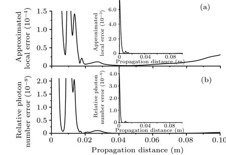
Fig.2.Plots of propagation distance-dependent error estimations between two consecutive computational steps for (a) approximate local error(Eq.(11)),and(b)relative photon number error(Eq.(16))in a constant step of 40 µm, with inset showing enlarged section to compare the small scale errors,and error estimations depicted with the same x axis to facilitate graph comparison.
From the above analysis, it can be concluded that when the waveforms in the time domain and in frequency domain change dramatically,the approximate local error curve and relative photon number error become large,so,the step should be reduced to produce a small error;otherwise,when the approximated local error and relative photon number error become small,step should be increased to reduce the simulation time.
Supercontinuum generation in a high-birefringence photonic crystal fiber (PCF) is also simulated with the same parameters by RK4IP-LEM with a relative local errorηG=10-6and RK4IP-CQE with a relative photon number errorηP=10-14.Figure 3 shows the calculation results.The output spectra calculated by three different methods are completely the same,which means that RK4IP-LEM and RK4IP-CQE are reliable.

Fig.3.Slow and fast axis output spectra of high birefringence PCF calculation by RK4IP,RK4IP-LEM,and RK4IP-CQE methods.
To make a comparison of accuracy and efficiency between the RK4IP-LEM method and the RK4IP-CQE method,the computational time value with the global error of the twoadaptive step-control algorithm is shown in Fig.4.The global average error in Fig.4 is defined as
where the complex field ˜Acalis calculated by the RK4IP-LEM method and the RK4IP-CQE method, ˜Aaccis calculated by the RK4IP in steps of 0.1µm.
It can be seen from Fig.4 that the computational time taken by each of the RK4IP-LEM method and the RK4IPCQE method generally decreases with the global average error increasing.However,the computational time taken by the RK4IP-LEM method is much more than that by the RK4IPCQE method,which is 30 times more than that by the RK4IPCQE method when the global average error is less than 10-7,and is about 20 times more than that by the RK4IP-CQE method when the global average error is more than 10-7.

Fig.4.Computational time taken by RK4IP-CQE and RK4IP-LEM against global average error, normalized by the time required to evaluate 103 FFT, for the supercontinuum generation process in highbirefringence PCF.
The RK4IP-LEM method uses one more FFTs than the RK4IP-CQE at each step as indicated in the above section.If the step sizes of two methods in each iteration process are the same, the computational time of RK4IP-LEM will be twice longer than that of the RK4IP-CQE method.In order to explain the difference in computational time between the RK4IPLEM method and the RK4IP-CQE method, the error estimations between the two consecutive steps for the approximate local error and relative photon number error are calculated by the RK4IP method in different step sizes,furthermore,the valuations of the step size and the error between two consecutive steps in calculation process of the RK4IP-LEM method and the RK4IP-CQE method under different error limits are also calculated.The results are shown in Figs.5-7,respectively.
Figure 5 shows the approximate local error and relative photon number error between two consecutive steps calculated by the RK4IP method in steps of 10µm,20µm,40µm,and 80 µm.As shown in Fig.5(a), the approximate local error curves are similar when the step size is 40 µm and 80 µm,respectively.They both fluctuate heavily in a propagation distance range of 0 m-0.05 m.When the pulse propagating distance is more than 0.05 m,the two error curves rise monotonically.The reason of the fluctuations can be found in Fig.2.While the step size decreases to 10µm and 20µm,the fluctuation between 0 m-0.05 m disappear,which is different from that in steps of 40 µm and 80 µm.As shown in Fig.5(b),except for different error amplitudes,the relative photon number curves are all nearly the same in steps of 80 µm, 40 µm,20 µm, and 10 µm.They all fluctuate heavily in the propagation distance of 0 m-0.05 m and rise monotonically for the propagation distance large than 0.05 m.

Fig.5.Variations of (a) approximated local error (Eq.(11)) and (b)relative photon number error(Eq.(17))with different propagation distances,calculated by RK4IP method in steps of 10µm,20µm,40µm,80µm,with y axis being logarithmic.
Figure 6 shows the variations of step size with the propagation distance in the process by using the RK4IP-LEM method and the RK4IP-CQE method under different approximate local error limitsηGand the relative photon number error limitsηPrespectively.In Fig.6(a), except small oscillations near 0.01 m and 0.02 m,the step size increases until the propagation distance reaches 0.05 m at the approximate local error limitηG=10-5.The step size decreases monotonically after 0.05 m.The small oscillations near 0.01 m and 0.02 m disappear gradually and the step size increases monotonically before 0.05 m and then decreases monotonically as theηGdecreases to 10-6,10-7,and 10-8.The smaller theηG,the more gently the change of the step size is.It is shown in Fig.6(b)that the step size curves with different relative photon number limitsηP=10-12; 10-13; 10-14, 10-15all oscillate heavily in a propagation distance range of 0 m-0.03 m; the step size increases monotonically in 0.03 m-0.05 m and the step size decreases monotonically in 0.05 m-0.1 m.

Fig.6.Step sizes versus propagation distances obtained by(a)RK4IPLEM)and(b)RK4IP-CQE under different error limits.

Fig.7.(a) Approximated local error of RK4IP-LEM and (b) relative photon number error of RK4IP-CQE between consecutive computational steps under different error limits.
Figure 7 is the approximated local error(Fig.7(a))and the relative photon number error(Fig.7(b))between the consecutive computational steps varying with the propagation distance in solving the C-GNLSE by the RK4IP-LEM method and the RK4IP-CQE method with different error limits.In Fig.7(a)the approximate local errors are all under the presetting error limits atηGequating 10-5,10-6,10-7,and 10-8.The fluctuations of the approximate local error curves become gentle as the change time of the step (ηG) decreases.In Fig.7(b), except within the propagation distance between 0.01 m-0.02 m,the relative photon number errors are all under the presetting error limits atηPequating 10-12, 10-13, 10-14, and 10-15.The fluctuations of the relative photon number error are nearly the same as those as theηPdecreases, which means that the change of the step is independent of the value ofηP.
From the above analyses, the difference between computational time taken by the RK4IP-LEM method and the computational time taken by the RK4IP-CQE method at the same global average error level in Fig.4 can be qualitatively explained by the results of Figs.5-7.Owing to the nonconserved qualitatively approximated local error,the approximated local error curves under different step sizes are not similar(see Fig.5(a)), which means that convergence rate of the approximated local error is much different from the error limitηGat every step of the propagation distance.The different convergence rates make the change of step size and approximated local error in the process of RK4IP-LEM different(see Figs.6(a) and 7(a)).The non-similarity of the change of the step size makes global average error of RK4IP-LEM not uniformly converge.However, the relative photon number error curves under different step sizes are similar because the relative photon number error is conserved quantity(see Fig.5(b)),and the change of step size and the relative photon number in the process of RK4IP-CQE method under different error limits are similar (see Figs.6(b) and 7(b)).The similarity of the changing of the step size makes the global average error of RK4IP-CQE method converge uniformly.The difference between the convergences of the relative photon number error and the approximated local error induces the large difference in computational time at the same global average error in Fig.4.
5.Conclusions
By mapping the C-GNLSE in the normal picture into the interaction picture in the frequency domain, the conservation quantity error adaptive step-control method and the local error adaptive step-control method are developed based on a vector form of the fourth-order Runge-Kutta in interaction picture.To prove the efficiency of the adaptive step-control methods, the two adaptive step-control methods and the RK4IP method are used to simulate the SC generation in the high birefringence PCF.The calculation accuracy and efficiency for each of these two adaptive step-control methods are discussed.At the same global average error, the computational time of RK4IP-CQE has been improved 20 times compared with that of RK4IP-LEM due to the convergences of the relative photon number error and the approximated local error.The methods will be useful for simulating the vector pulses transmission and the supercontinuum generation in the nonlinear fiber and waveguides, the pulse propagating in the multimode optical fiber,and the interaction between different pulses.
Appendix A
LetAnbe the pulse envelope for the polarizationn, then the photon numberPduring propagation will be defined as

Calculating each integral term in Eq.(A3),the following equation are obtained:
LetΩ=ω1,Ω1=ω,Ω2=ω2+ω1-ωand use the expression ofRn(Ω1-Ω)=R∗n(Ω-Ω1), then equations(A4)and(A5)will change into Eqs.(A8)and(A9),i.e.,
Substituting Eqs.(A6)-(A9)into Eq.(A3),then the expression of∂P/∂z=0 is obtained.
Acknowledgement
Project supported by the National Key Research and Development Program of China (Grant Nos.2021YFC2201803 and 2020YFC2200104).
猜你喜欢
作文小学高年级(2023年1期)2023-03-13
光明中医(2022年22期)2022-12-29
农业环境科学学报(2022年11期)2022-12-02
中国宝玉石(2021年5期)2021-11-18
初中生学习指导·中考版(2020年2期)2020-09-10
初中生学习指导·中考版(2020年3期)2020-09-10
北方音乐(2020年7期)2020-06-01
中华诗词(2019年1期)2019-08-23
中华诗词(2018年5期)2018-11-22
中华诗词(2018年1期)2018-06-26

- Chinese Physics B的其它文章
- Matrix integrable fifth-order mKdV equations and their soliton solutions
- Comparison of differential evolution,particle swarm optimization,quantum-behaved particle swarm optimization,and quantum evolutionary algorithm for preparation of quantum states
- Explicit K-symplectic methods for nonseparable non-canonical Hamiltonian systems
- Molecular dynamics study of interactions between edge dislocation and irradiation-induced defects in Fe-10Ni-20Cr alloy
- Engineering topological state transfer in four-period Su-Schrieffer-Heeger chain
- Spontaneous emission of a moving atom in a waveguide of rectangular cross section