Electrical properties of a generalized 2 × n resistor network

Shi Zhou,Zhi-Xuan Wang,Yong-Qi Zhao and Zhi-Zhong Tan

Department of physics,Nantong University,Nantong 226019,China

Abstract

Any changes in resistor conditions will increase the difficulty of resistor network research.This paper considers a new model of a generalized 2 × n resistor network with an arbitrary intermediate axis that was previously unsolved.We investigate the potential function and equivalent resistance of the 2 × n resistor network using the RT-I theory.The RT-I method involves four main steps:(1)establishing difference equations on branch currents,(2)applying a matrix transform to study the general solution of the differential equation,(3)obtaining a current analysis of each branch according to the boundary constraints,and (4) deriving the potential function of any node of the 2×n resistor network by matrix transformation,and the equivalent resistance formula between any nodes.The article concludes with a discussion of a series of special results,comparing and verifying the correctness of the conclusions.The work establishes a theoretical basis for related scientific research and application.

Keywords: generalized network,difference equations,matrix transform,potential function,equivalent resistance

1.Introduction

The well-known nodal current and loop voltage laws were established by Kirchhoff in 1845;since then,great progress has been made in the research and application of resistor networks[1].When solving some complex scientific problems,the use of resistor network models can make the problems specific and intuitive,and easy to analyze and study.Therefore,the resistor network model has certain practical value for scientific research.For example,the study of the resistance between two points of an infinite grid and some new ideas and methods were proposed in references [2-4].In particular,in 2000,Prof.Cserti made great progress and proposed the lattice Green’s function to calculate the resistance of infinite resistor networks [3],providing an effective method for many scholars who study the resistance of an infinite resistor network.Green’s function is a very important theoretical tool for computing infinite networks,as shown by the excellent applications of the theoretical works in reference[3]on the study of the infinite network.Giordano[4],Asad[5],Asad and Hijjawi[6-9],Owaidat[10-15],and Cserti et al [16] have also made new theoretical achievements.The application of Green’s function is a very efficient way to find the resistance of an infinitely resistive network.But the infinite resistance network model is always idealized,and the finite resistance network is the actual real-life problem.Obviously,Green’s function does not apply to finite resistor networks.However,Wu [17] proposed a different method (called the Laplace matrix method) in 2004 and used the eigenvalues and eigenvectors of the Laplace matrix to calculate the resistance between any two nodes in a resistor network.This method is used to calculate the resistance between any nodes of the finite resistance lattice and has made a significant contribution to the study of the finite resistance network model.Laplace matrix analysis has also been applied to impedance networks in the literature [18].Later,Chair [19] and Chair and Dannoun [20]used Wu’s results to study the simple random network and the single-sum problem of the Möbius n-ladder network,simplifying the results of the double sum.After some improvements,the Laplace matrix method was further developed and applied[21,22].The Laplace matrix method relies on two matrices in two directions and is not suitable for networks at arbitrary boundaries.

How to solve the problem of the resistance network with an arbitrary boundary is a longstanding scientific problem.However,in 2011,there was a turning point,Tan proposed a new theory to solve this problem.Tan’s theory only relies on one matrix in one direction [1],which can avoid the eigenvalue problem of solving another matrix,and allows having any element in the other matrix (because the theory does not need to solve it).In 2015,Tan called the method the recursion-transform (RT) method [23-25].At that time,the RT method took the branch current as the parameter to establish the matrix equation,so it is also called the RT-I method.In 2017,Tan also established the method of establishing a matrix equation with node voltage as a parameter,which is called the RT-V method [26].The RT theory can not only calculate the equivalent resistance but also conveniently solve the potential function,Tan and Tan et al used RT theory to solve many resistor network problems of various complex structures [27-38].RT theory combined with variable substitution technology can also conveniently study complex impedance problems.In the RT theory,there is a special method called the N-RT method,which specializes in studying the equivalent resistance of n-order circuit networks.In practical applications,n-order circuit networks have very important research value [39-41].For example,in the literature [39,40],equivalent circuits can be used to study the reflection and refraction of electromagnetic waves of the superstructure grating,while reference [41] uses complex impedance circuits to study water transport in plants.At present,researchers have accomplished many achievements in research by using the N-RT method [42-49].This paper intends to study a class of a generalized 2×n circuit network model,which is different from previous models in that the resistance on the middle axis is independent of the resistance on the upper and lower boundaries as shown in figure 1.We use the RT-I approach for this problem.We use the RT-I method to study the analytical expression of the electrical characteristics of this circuit network (node potential and equivalent resistance).

Figure 1.A generalized 2 × n resistor network with an arbitrary intermediate horizontal axis; there are three resistance elements {r0,r,r1}arranged in the network model.

This article is organized as follows: in section 2,a series of major results on the 2 × n resistor network are presented(including the potential function formula for any node and the equivalent resistance formula between any nodes).The methods and calculations used in this study are described in section 3.Section 4 presents the main results.And in section 5,we provide a number of special cases,while comparing and verifying their correctness.

2.Main results

We define a generalized 2 × n resistor network with an arbitrary intermediate horizontal axis as shown in figure 1.There are three resistance elements{r0,r,r1}arranged in the network model,and the resistancer1is located on the middle horizontal axis,the resistanceris located on the upper and lower boundary lines,and the resistancer0is located on the vertical axis.Set the horizontal line as the X-axis,and assume current J from theAx1input and from thePx2(Px2=Cx2,Bx2,Ax2) output (without loss of generality letx1≤x2).Set the potential function of any noded(x,y) toU(x,y),selectingU(B0) as the potential reference point.The above assumptions apply throughout this article.

2.1.Necessary parameter definitions

The content of this article is complex,and there are many equations and parameters,so in order to facilitate the research and calculations,and to simplify the various expressions given below,the following definitions are given:

The above parameters are important to use in this article and applicable throughout the article.

2.2.Analytic expression of the potential function

Consider a generalized 2 × n resistor network shown in figure 1,let current J flow fromAx1toCx2(x1≤x2).SelectU(B0) as the potential reference point,and set the horizontal line as the X-axis,the potential function formulae of the 2×n circuit network are as follows:

(a) The potential function of the nodeAxon the axisA0Ancan be expressed as

whereh=is defined in equation (5),andxsis a piecewise function

(b) The potential function of nodeBxon the axisB0Bncan be expressed as

In particular,whenx=0,the potential of the reference pointU(B0)=U0is obtained as

(c) The potential function of nodeCxon the axisC0Cncan be expressed as

The above potential function formula is given for the first time in this paper,which is a theoretical innovation and discovery.Note thatB0is chosen as the potential reference point in all of the above conclusions,andU(B0) is given by equation (9).

2.3.Equivalent resistance formulae

Consider a generalized 2 × n circuit network as shown in figure 1,set the horizontal line as the x-axis,and the equivalent resistance betweenAx1andCx2can be expressed as

where 0≤x1≤n,0≤x2≤n,andis short for,which is defined in equation (5).

The equivalent resistance betweenAx1andAx2can be expressed as

Formulas(11)and(12)are given for the first time in this article and are applicable to cases wherex1,x2,nare any natural numbers,and also cases wherenis infinite(this issue will be discussed later in this article).

In the following,we use RT-I theory to give a detailed calculation process of all the above conclusions.RT-I theory is an advanced theory established in the literature [23] to study the resistor network model and mainly consists of four basic steps:first,establishing a matrix equation of the current parameters on three adjacent vertical axes; second,establishing a boundary condition of the current parameter; third,implementing a diagonal matrix transformation to solve the matrix equations;and fourth,implementing the matrix inverse transformation to solve the branch current,calculate the node potential,and find the equivalent resistance.

3.Methods and calculations

3.1.Modeling general differential equations

As shown in figure 1,below we use RT-I theory to carry out our research.Let current J flow from nodeAx1to nodeCx2(orAx2).For ease of study,we show a network graph in figure 2 with current parameters and their directions.Let the currents passing through the three rows of horizontal axis resistors beIak,Ibk,Ick(1 ≤k≤n),and the currents passing through the vertical resistancer0areIkandI′k(0 ≤k≤n).

Using Kirchhoff’s loop voltage law,the current equations for the kth grid are obtained as

Similarly,the current equation of the (k+1)th grid loop can be obtained.Then,taking the difference between the equations obtained and equations (13) and (14),we get

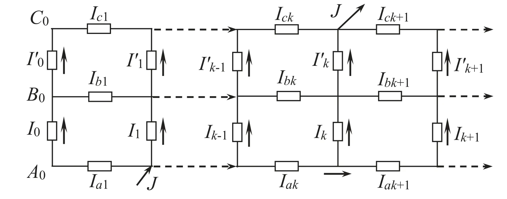
Figure 2.Sub-network of a 2 × n resistor network with current parameters.

By the Kirchhoff node current equation shown in figure 2,we can get

Substituting equations (17) into (15) and (16),respectively,and simplifying them,we can get

Research shows that it is difficult to obtain a direct solution to the systems of equations(18)and(19);thus,we use the RT-I theory to express equations (18) and (19) as the matrix

whereh=The key step in RT-I theory is to do a matrix transformation to indirectly study the general solution.The specific transformation method is to implement a diagonal matrix transformation for the second-order matrix in (20).For example,

Assume that there are constantst1,t2and elements of [1,pi],

which satisfy

Equation(22)is regarded as the identity matrix and is solved to obtain

Equation(24)is the definition given in equation(2)above.So equations (23) and (24) can convert the matrix equation (21)into a new matrix equation,

where the transformation relationship is

Let the two roots ofx2-tix+1=0from (25) beλk,(k=1,2),by solving the characteristic equation we have equation (3).

Equation(25)is the simple linear difference equation,so solving the difference equation (25) results in a segmented function solution,

3.2.Constraint equations on the left and right boundaries

According to RT-I theory[23],the constraint of the boundary current has four parts,namely,the leftmost and rightmost boundary conditions,and the boundary condition at the input and output current.First,consider the current constraint of the left boundary grid.According to figure 2,the first loop voltage equations can be obtained as

And we get the node current equationsIb1=I0-I0′,Ia1=-I0,Ic1=I0′.From these equations,one can get

Next,we useP2×2appearing in equation (21) to multiply equation (31) to implement the matrix transformation; then,the matrix equation (31) can be transformed into

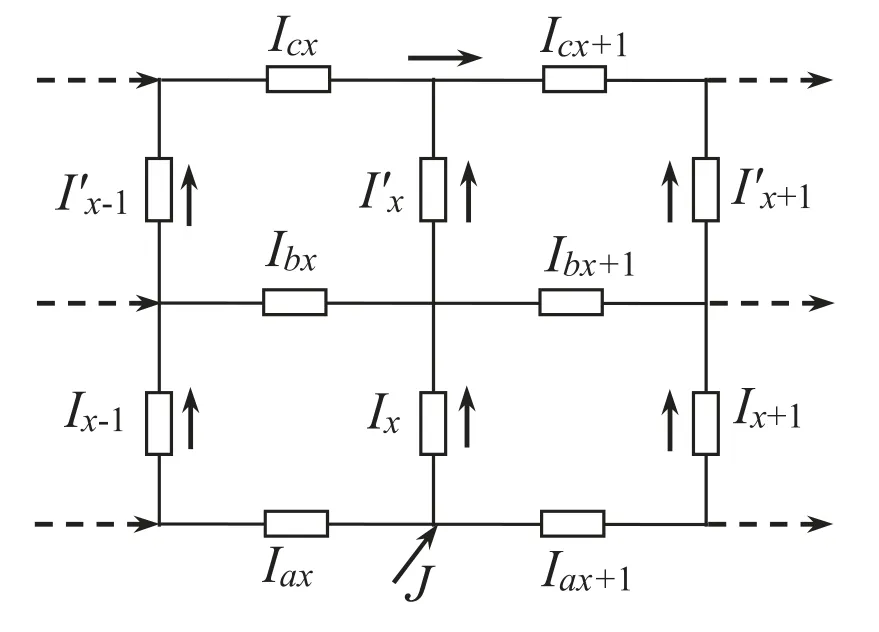
Figure 3.Current input image with the current parameters of the 2 × n resistor network.

wheretiis given by equation (24).

Secondly,consider the constraint equation of the right boundary grid.Similar to the establishment of equation (31),we have

Similar to the matrix transformation above,the matrix equation (33) can be transformed into

The above equations are general-purpose equations for all cases and can be applied to calculate potential functions in various situations.The following are special current constraint equations based on different current output conditions.

3.3.Constraint equation of the current input and output

First,we consider the case of input current J at nodeAx1.Similar to the network analysis method above,from figure 3,we can obtain a matrix equation in the case of node current input

Let us take the matrix that appeared in(21)times the matrix(35)from the left to do the matrix transformation,then the matrix equation (35) can be transformed into

Second,we consider the case of the input current at nodeCx2.The matrix equations are obtained using the same method described above,

Similar to the matrix transformation we did above,the matrix equation (37) can be transformed into

wherepi={1,-1}is given by equation (23).

In addition,if we consider the case of output current from the nodeAx2,the difference equation can be rewritten as

The above series of equations (20)-(39) are all the equations we need,and based on these equations,the analytical formulae (6)-(12) can be derived.The detailed calculation process is given below.

4.Derivation of main results

4.1.A general solution of the matrix equations

In order to derive the analytical formula of the potential function,a potential reference point needs to be set.Let nodeB0be the potential reference point,and setU(B0)=U0.Because the potential decreases along the current direction,the potential functions on any axis are

where 0≤x≤n,and the currentI′xandIxare shown in figures 2 and 3.

Next,to calculate the currentIbk,the analytical formula of the matrix equationXk(i)needs to be solved first.Substituting(32) into (27) to get (0≤k≤x1)

Substituting (43) into (28) to get (x1≤k≤x2)

Substituting (43) withk=x1,x1-1into (44),yielding(x1≤k≤x2)

Substituting (38) into (29),we can get (x2≤k≤n)

Substituting (45) withk=x2,x2-1into (46),yielding (x2≤k≤n)

Substituting (47) withk=n-1,ninto (34),and simplifying it we get

This is a key solution on which all ranges of solutions depend.Therefore,substituting equation(48)into equations(43),(45),and (47) to get a general formula,

4.2.Calculate the branch currents

Applying the matrix inverse transformation by the matrix equation (26),one can get

In addition,the node current equationIbk-Ibk-1=Ik-1-Ik′-1is obtained according to figure 2,and then we use equation (50) to get

For the following potential function to be derived,we need to calculate equation (54) in sections.

When 0≤k≤x1,substituting equation (43) into equation (51) we get

Summing over equation(52)again,one can get(0≤k≤x1)

whereXk(i)is given by equation (49).

Whenx1≤k≤x2,substituting equation (45) into equation (51),we get

Further,the sum is calculated as

Whenx2≤k≤n,substituting equation (47) into equation (51),we get

Utilize equation (55) and further calculate equation (56) to obtain (x2≤k≤n)

whereXk(i)is given by equation (49).

Sincet2-2=h+2h1,the above equations can be rewritten uniformly as

wherexs={x1,x≤x1} ∪{x,x1≤x≤x2}∪{x2,x≥x2}is defined in equation(7).Equation(58)is a key equation for calculating voltages,which can be conveniently applied to equation (40) to solve the potential function.

4.3.Derivation of the potential functions

Substituting equation (58) into equation (40),we get

Let the potential reference point be B0,and the reference potential isso equation(59)can be rewritten as

whereXk(i)is given by equation (49).Note that equation (60)is self-consistent with the assumption ofU(B0)=U0,because there must beU(B0)=U0whenx=0.

We can immediately derive the potential function (8)when substituting equation (49) into equation (60).Here we first prove the potential function (8).

In addition,the potential function(6)can be obtained by equation (41) and equation (50) as

Substituting equation (60) into equation (61) and simplifying it

whereXk(i)is given by equation (49).Substituting equation (49) into equation (62),the potential function (6) is derived.

Finally,by calculating the potentialU(Cx) by equations (42) and (50),one can get

Substituting equation (60) into equation (63) and simplifying it,we have

Substituting equation (49) into (64),we immediately derive the potential function (10).

So far,the analytical formulae of the potential function are fully proven.The above proof process is logical and the results are self-consistent.

4.4.Derivation of equivalent resistance

Next,we derive the equivalent resistance of equations (11)and (12).When calculating the equivalent resistanceR(Ax1Cx2),equations (6) and (10) can be used directly.For example,takingx=x1in equation (6) andx=x2in equation (10),respectively,one can get

Using Ohm’s lawR(Ax1Cx2)=[U(Ax1)-U(Cx2)]/J,then by equations (65) and (66) derive equation (11).

In addition,when deriving the equivalent resistanceR(Ax1Ax2),it is necessary to reconsider the situation in which current J flows fromAx1to nodeAx2,in this case,except for equations (37) and (38),the remaining equations (13)-(36)and equations(40)and(42)are general equations suitable for all cases.To calculate the equivalent resistanceR(Ax1Ax2),simply replace equation (38) with equation (39).

Similar to the derivation of equations (48) and (49)above,by equations (27)-(29),(32)-(36),and (39),one can get

and obtain (x1≤k≤x2)

By figure 2,one can compute the voltagesU(Ax1,Ax2)that go through three different paths,

The upper three forms are appropriately deformed and summed to get

According to the continuity equation of the currentIai+Ibi+Ici=J,substituting it into equation (70),one can get

Substitute equation (50) withk=x1,x2into equation (71) to yield

When equation (68) is taken ask=x1,x2,respectively,substituting equation (68) into equation (72),one can get

When applying equation (73) to Ohm’s lawRn(Ax1,Ax2)=U(Ax1,Ax2)/J,the resistance formula (12) is derived.

So far formulae (11) and (12) are proved.The following are several special cases of electrical characteristics,also compared and studied for their correctness.Of course,since all the calculations in this article are rigorous and precise,and all the results are self-consistent,the results presented must be correct.

5.Special cases and comparisons

The potential functions and two equivalent resistance formulae of a generalized 2 × n resistor network are given above.Since the model shown in figure 1 has three arbitrary independent parameters of {r,r0,r1},all the formulas presented in this article have universal applicability and represent all situations.Some of their special cases are given below,while comparing and verifying their correctness.

Example 1.In the network shown in figure 1,let current J flows fromAx1toCx2,selectU(B0) as the potential reference point,then by equations (6) and (10),one can get a potential function relationship,

whereh=r/r0,h1=r1/r0,andxsis a piecewise function given by equation (7).

Example 2.From equations (8) and (74),we get a potential function relationship (0 ≤x≤n)

Equation (75) is an interesting function relation,particularly when0≤x≤x1,using equation (75) to get

Example 3.In the network shown in figure 1,let current J flow fromAx1toCx2,then equations (6) and (10) are subtracted to give the potential function relationship

Equation (77) reveals a simple relationship between two voltages.

Example 4.In the network shown in figure 1,from equations (11) and (12),one can get a formula relationship between two different equivalent resistances,

Equation(78)is an interesting relational equation that reveals the intrinsic relationship between two equivalent resistances.In particular,whenn→∞ butx1,x2are finite,from equation (78) we have

Example 5.Whenr1=r,the equivalent resistances equations (11) and (12) degrade to the following simple results:

Reference [1] has studied the equivalent resistance.Whenr1=r,comparing the results in [1] with our results of equations(80)and(81),it is not difficult to find that they are exactly the same,which verifies the correctness of the conclusions obtained in this paper.

Example 6.Consider the case ofx2=x1,andx1=0,x2=n,three formulae are derived from equations (11) and(12),respectively

Example 7.Whenr1=∞,from equations(11)and(12),one can get

Example 8.Whenr1=0,it leads toh1=0,from equation (2) to gett2=t1=2+h,soλ2=λ1,and=,then equations (11) and (12) degrade to

Example 9.Consider the case of a half-infinite resistor network.Whenx1,x2is finite butn→∞,there is a limit of

Whenr1=r,taking the limits of equations(11)and(12),one can get the equivalent resistance formulas for two infinite networks:

where we define

In particular,whenx1=x2=x,equation (90) degrades to

whereh=

6.Summary and comments

This paper considers a generalized 2 × n network shown in figure 1,and uses RT-I theory to study the electrical properties (potential function and equivalent resistance) of a class of 2 × n resistor networks with an arbitrary intermediate resistance axis.This is of great significance for the study of the 2 × n resistor network model with multiple parameters.The main results of the research presented in this paper are potential functions of any node of a 2 × n resistor network such as equations (6),(8),and (10),and two equivalent resistance formulae such as equations (11) and (12).Equations (6)-(12) are given for the first time in this paper and are a theoretical innovation and discovery.Besides,they are universal,applicable to cases wherex1,x2,nare any natural numbers,and also to cases wherenis infinite.In addition to studying the generally applicable cases,this paper also gives some special situations and compares and verifies the correctness of the conclusions.By discussing a series of special results,several interesting relational formulas were also obtained.In general,the work in this paper provides several new and universally applicable theoretical formulas for the study of the resistor network model.

Also,the basic formula obtained in this paper is also applicable to the structure of the complex impedance network shown in figure 1,and only the complex impedance needs to be replaced with the complex impedance,so that the general expression of the equivalent complex impedance of any node of the 2 × n impedance network can be obtained directly.

Acknowledgments

This work is supported by the National Training Programs of Innovation and Entrepreneurship for Undergraduates (Grant No.202210304006Z),and supported by the Jiangsu Training Programs of Innovation and Entrepreneurship for Undergraduates (Grant No.202210304076Y).

Author contributions

S.Z.investigated the research background of this problem;Z-X.W.drew images from the text and checked the syntax;Y-Q.Z.checked and validated the correctness of the calculations; Z-Z.T.designed the research and performed the theoretical calculation and analysis,and also wrote the first draft of the article.

Data availability statement

No Data associated in the manuscript.

ORCID iDs