
Application of Newtonian approximate model to LIGO gravitational wave data processing
2023-10-11 07:55JieWu吴洁JinLi李瑾andQingQuanJiang蒋青权
Chinese Physics B 2023年9期
Jie Wu(吴洁), Jin Li(李瑾),†, and Qing-Quan Jiang(蒋青权)
1College of Physics,Chongqing University,Chongqing 401331,China
2Department of Physics and Chongqing Key Laboratory for Strongly Coupled Physics,Chongqing University,Chongqing 401331,China
3School of Physics and Astronomy,China West Normal University,Nanchong 637009,China
Keywords: gravitational waves,black holes,matched filtering,data fitting
1.Introduction
At the beginning of the 20th century,Albert Einstein put forward General Relativity and predicted the existence of GW.In the next hundred years, scientists have been committed to verifying this prediction theoretically and experimentally.[1,2]In 2015, Advanced LIGO began to observe the GWs from 20 Hz to 1 kHz frequency band.[3]Two advanced laser interferometer GW detectors located in Hanford and Livingston simultaneously detected GW event GW150914, which directly verified the existence of GW for the first time.[4]In the next few years, nearly 100 GW events involving the mergers of compact binary systems were successfully detected,including two binary neutron star(BNS)events,[5,6]which led to the development of multi-messenger astronomy and opened the new era of GW astronomy.[7–10]How to detect and analyze GW signals quickly and accurately has become one of the research focuses of GW data processing.[11]
The construction of theoretical templates is crucial for the data processing of GW generated by compact binary coalescence (CBC).At present, the most accurate template is from the effective-one-body model[12,13]based on the algorithm of numerical relativity(EOBNR).[14–16]The parameter space dimension corresponding to this model is 9 at least,[17,18]so using EOBNR for matched filtering requires huge computing resources.At the same time, parameter estimation is also essential in GW data processing.The commonly used parameter estimation methods[19]include maximumlikelihood estimation,[20]Markov chain Monte Carlo,[21]nested sampling,[22]machine learning,[23]etc.These methods also require huge computing resources.We try to build an analytic waveform through a low-order approximate model,and determine the coalescence time in LIGO segments containing GW signals based on matched filtering,then estimate the chirp mass of the GW source through sampling and fitting the analytic frequency curve with the preprocessed time-frequency spectrogram.The low-order approximate model can quickly process segments containing GW events, which only need a few computing resources and time.The average chirp mass of BBH events is 22.05M⊙, which is ideal and close to 23.80M⊙given by the Gravitational Wave Open Science Center(GWOSC),[24]which has certain research value for fast and accurate analysis of GW data.
2.Template construction: Newtonian approximate model
At present,the structure and mechanism of the GW generated by CBC are relatively clear.[25]The whole process generally evolves in three different phases: inspiral, merger, and ringdown.[26,27]In addition to EOBNR, the post-Newtonian approximation is also commonly used to construct theoretical templates.[28,29]The inspiral and merger phases of the NA model used in this paper belong to the lowest-order Newtonian approximation, without considering the effects of spin,precession, and redshift on the waveform.This work mainly refers to the low-order Newtonian approximation describing CBC in Refs.[30–32],and improves it to build the NA model.In the inspiral and merger phases, the low-order approximate method is used to treat the compact binary system as a particle.And in the weak field limit, we can describe spacetime with a weak perturbation asgµν=ηµν+hµνand the wave solution corresponding to Einstein’s field equation is solved by it.The mass quadrupole is introduced to solve the gravitational radiation,[33]and the GW waveformh(t)and frequency curvef(t)with radiated energy are solved through coordinate transformation.In the ringdown phase,we construct the model by treating the strain as exponential decay and keeping the frequency basically unchanged,which is helpful to determine the coalescence time and provide the initial chirp mass in Section 4.[34,35]Finally, we combine these things to construct a low-order GW theoretical template conforming to CBC.
Settcas the coalescence time,andτ=tc-tis the time to coalescence.The positive and negative values ofτrepresent the time before and after the coalescence time.The specific waveform is as follows:
where
F×andF+are the antenna response functions for the incident signal,[36,37]
is the chirp mass of the GW source,m1andm1are the masses of binary system,Dis the luminosity distance,ιis the inclination angle,Φ0is the coalescence phase, andδis a small quantity to prevent the waveform and frequency from infinity whenτ=0.In this paper,we set
In the NA model,the compact binary system is regarded as a particle, which is feasible in the inspiral phase, but it cannot be regarded as a particle in the merger and ringdown phases,otherwise,it will produce a large deviation.Therefore,the attenuation term is added to it to make it close to the model of EOBNR at all phases,which can meet the basic requirements for determining the GW signal and parameter estimation.Theoretically,the NA model is applicable to CBC.However,due to the lack of data stream preprocessing and inadequate sampling of parameter estimation,we only apply the NA model to BBH instead of BNS.The results of its application to BNS are described in Section 5.
To verify the accuracy of the NA model, it is compared with EOBNR.It can be seen from Fig.1 that in the waveform,the GW strain increases with time.The strain of the NA model and EOBNR change the same.Although there is a slight difference in the phase, it is sufficient for the preliminary determination of the signal position.We will discuss the bias in the estimation caused by the phase in Subsection 4.2.For the frequency curve, as it approaches the coalescence time, the frequency curve grows faster and faster.In the inspiral phase,the frequency curve of the NA model is slightly higher than that of EOBNR,which can also be seen from the phase change of the waveform, while the merger and ringdown phases almost coincide.Since the detected GW signals are most apparent before the coalescence time,and the frequency curve of the NA model can be well-matched during this period,we will use this frequency curve for parameter estimation later.The velocity of the binary system gradually increases,the separation gradually decreases,and the curves of the NA model and EOBNR are also very close.As the coalescence time approaches, the curves almost coincide.
The three GW events shown in Fig.1 represent systems with different chirp masses and different distances, while the GW templates described by the NA model and EOBNR under different parameters are very close, which shows the feasibility of constructing the GW template by low-order approximate model.In the NA model,the elliptical orbit of compact binary systems will rapidly circularize through the numerical solution, so the eccentricity of the orbit does not need to be considered.[42–45]At the same time, as a low-order approximate model, the NA model does not consider the effects of redshift,spin,precession,and other effects.Note that the purpose of using the NA model is to match it with detected data containing known GW events,determine the coalescence time and provide initial chirp mass for fitting, rather than replace the existing EOBNR to detect GW.
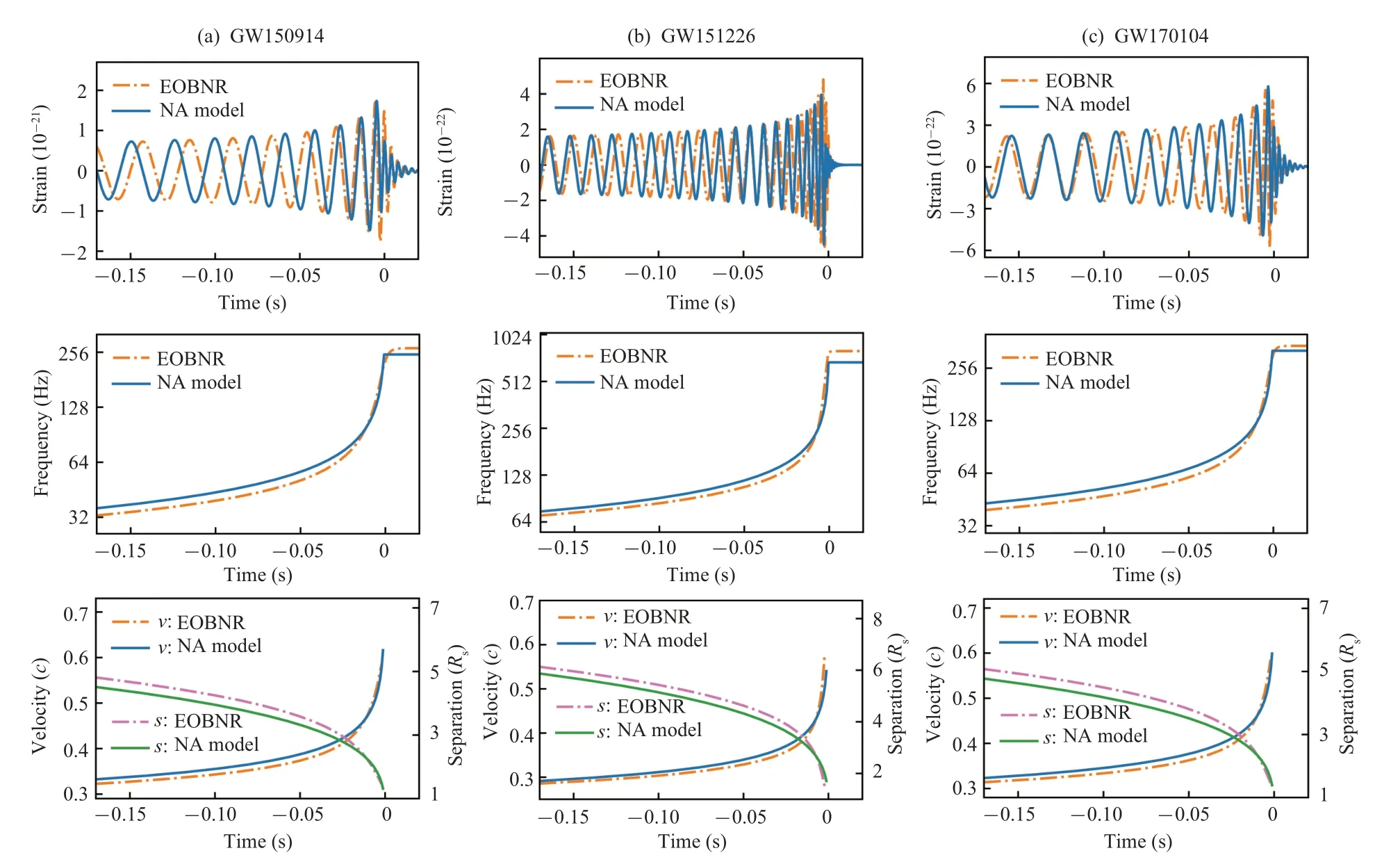
Fig.1.Comparison of the NA model and EOBNR for GW159014,GW151226,and GW170104.The NA model and EOBNR are compared in four aspects:waveform,frequency curve,velocity,and separation.The solid lines represent the NA model,and the dotted lines represent EOBNR.The effective relative velocity and the Keplerian effective separation are in units of the speed of light and Schwarzschild radii which are given by post-Newtonian parameters v/c=(GMπ f/c3)1/3 and R/Rs=Rc2/2GM,where M is the total mass.The chirp masses given by GWOSC are 28.6,8.9,and 24.1 M⊙and the luminosity distances are 440,450,and 990 Mpc.[38–40] The simulations of EOBNR are from PyCBC.[41]
In order to verify the efficiency of the NA model generation, we compare several common GW models and obtain the results in Table 1.It can be seen that the NA model is extremely fast in terms of the model generation rate, and the accuracy of the NA model is completely sufficient for the processing flow used in our paper.Therefore,the NA model can be used to analyze GW data quickly.
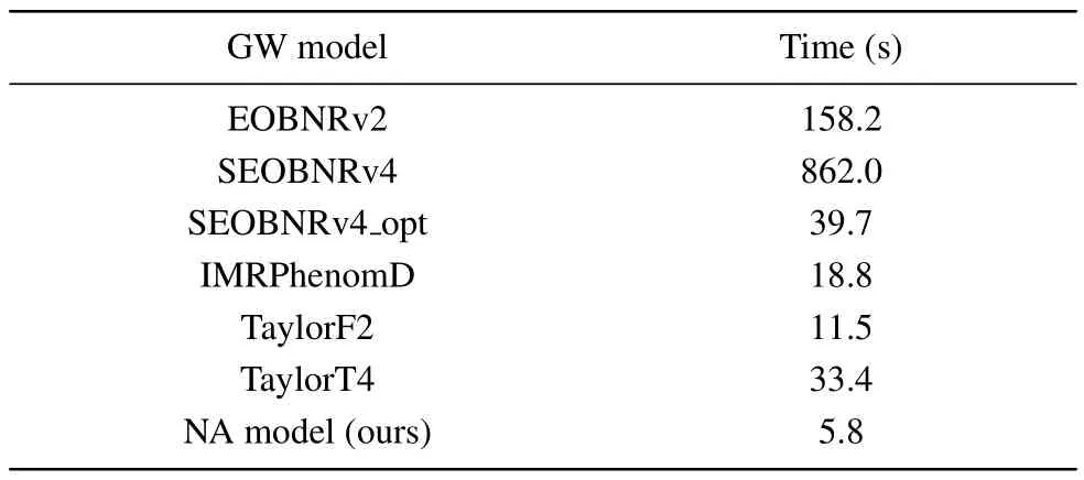
Table 1.Time comparison of generating signals by different GW models.Different models simultaneously generate 1000 GW signals with the same parameters, all of which are 10-s long in 4096-Hz sampling rates.All the GW models are from PyCBC.
3.GW data stream preprocessing
As the second generation of ground-based GW detectors,LIGO and Virgo detect GW through responding to the length of arms changes caused by GW.[46,47]But in addition to GW,many factors, such as the detector itself and the ground environment,will also lead to changes in the length of arms,so there are a lot of noises in the output data of the detector.These noises mainly include quantum sensing noise, seismic noise,suspension thermal noise, mirror coating thermal noise, and gravity gradient noise.[48]The signal preprocessing methods used in this paper are the most common methods: whitening data and wavelet transform.The basic signal processing steps are as follows:[49]
The noise in LIGO is approximately stationary and can be easily characterized in the frequency domain.The first step of data processing is to use fast Fourier transform (FFT) to convert raw data from the time domain to the frequency domain,and whiten the data by dividing the Fourier transformed data by the noise amplitude spectral density.Then,the 30 Hz–600 Hz part of the signal is retained after the filter to remove the low-frequency seismic noise and high-frequency quantum sensing noise,and the visibility of the signal in this frequency band is enhanced.Using inverse fast Fourier transform(iFFT),the signal processing in the frequency domain is retranslated to the time domain.
Continuous wavelet transform(CWT),like Fourier transform,is often used in signal analysis and data processing.Its basic idea is similar to the windowing of short time Fourier transform(STFT),and its window size can adaptively change.By using finite and decaying wavelet bases,it replaces the infinite triangular function bases in STFT, which is more conducive to time–frequency analysis of signals.We use the most widely used Morlet wavelet to convert signals from time domain to time-frequency spectrogram.
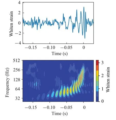
Fig.2.Results for preprocessing of GW150914(H1).H1 and L1 represent detectors of LIGO in Hanford and Livingston.Obtain the GW waveform and time-frequency spectrogram through whitening and wavelet transform.The strain in the waveform represents the relative strain after whitening,and the color of the time-frequency spectrogram represents the absolute whiten strain.
The result of GW150914 (H1) is shown in Fig.2.Note that in the following Figs.2–4, the processing results of H1 are all displayed,but the processing results of L1 are not displayed.This is because it is only used as an example to illustrate each processing flow,and in actual processing(see Subsection 4.3),both the H1 and L1 data are processed simultaneously.
In the time–frequency spectrogram,the GW signal is pronounced,and its frequency rises rapidly from 35 Hz to 350 Hz in a very short time.In Section 4, we will discuss how to use the time–frequency spectrogram to estimate the chirp mass through fitting the frequency curve.
4.Data analysis
4.1.Signal determination and parameter estimation
In the present work, the purpose of analyzing the LIGO GW data is to estimate the chirp mass of BBH.The differences from the traditional parameter estimation are described in the following.
(i) We use the simplified CBC GW waveform to determine the coalescence time of the GW events through matched filtering, so as to provide the initial chirp mass for the data fitting.
(ii) The chirp mass is estimated by fitting the time–frequency spectrogram near the coalescence time with the theoretical frequency curve.
Matched filtering is a common signal processing method that analyzes a signal by matching the signal to a known theoretical waveform.Among numerous GW sources,the physical process of the CBC releasing GW has been systematically studied, and the theoretical waveforms are largely clear (the case of BNS needs further correction).Therefore, this is the method used by LIGO to detect GW of CBC.In the matching process, millions of GW templates are matched and filtered with the output data from the detectors.After generating triggers by thresholding and clustering the SNR time series, the GW events and their time series ranges are locked after coupled event analysis and testing the hypothesis, and then estimate the parameters.[50,51]As the template of matched filtering, EOBNR has multiple parameters and requires complex numerical calculation,which requires huge computing resources.The NA model used in this paper,as a low-order approximate model,does not need to consider too many parameters and does not require huge computing resources in the process of the matched filtering.For the waveform,the template bank is constructed using the NA model.In Fig.3, based on the idea of the matched filtering,the template is matched with the raw data stream of the known GW events, and the point with the largest SNR is selected as the best matching point.The time corresponding to this point is the coalescence time of the GW event,and the chirp mass used for matching is the initial chirp mass of the next step for data fitting.Note that here the NA model is only used to determine the coalescence time and initial chirp mass,and cannot replace the current EOBNR for the GW detection.
Using the coalescence time and initial chirp mass determined above,the sampling points of the time–frequency spectrogram are estimated by data fitting.By adjusting the parameters of the theoretical curve, a number of discrete points are consistent with the theoretical curve, and the corresponding parameters are estimated.The basic method of data fitting is the ordinary least squares.The objective function of the optimization problem is to minimize the sum of squares of errors between the sampling value and the fitting function.Since the frequency curvef(t)described in Eq.(4)is only related to the parameter of chirp massℳ, we can estimate the chirp mass by fitting the frequency curve with the time–frequency spectrogram.In Fig.4,sample the GW signal in the spectrogram,select the points and then filter out those smaller thanktimes maximum point in the spectrogram, wherekis the sampling scale coefficient.Andkis like a percentage,which obviously belongs to[0,1].A larger value ofkindicates fewer sampling points.The frequency changes are extracted from the time–frequency spectrogram, and these sampling points are fitted with the frequency curve of the NA model to estimate the parameters of the chirp mass.
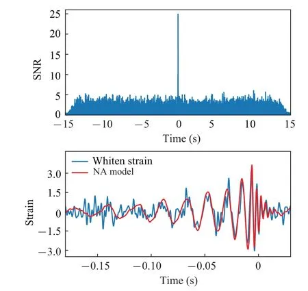
Fig.3.Result of matched filtering for GW150914(H1)after preprocessing in Fig.2.The specific coalescence time of GW events is determined based on matched filtering,where the signal-to-noise ratio(SNR)reaches 24.9.
Through the above processing flow,the processing result of GW event GW159014(H1)is shown in Figs.3 and 4.The GW signal and the waveform template match well,especially before and after the coalescence time,the GW signal is more evident than the background noise.The GW signal in the spectrogram is very prominent in the background noise, and there is an apparent change in the coalescence time.The frequency curve drawn by the NA model can conform to GW signal changes well, and it is feasible to determine the chirp mass through data fitting.Note that the NA model matches GW150914 very well,and the SNR of H1 is even close to 26 given by GWOSC.For the other events, the SNR is not too close to the values given by GWOSC.That is because when designing and improving the NA model, GW150914 and its EOBNR are used as references to adjust some parameters in the NA model,resulting in a high degree of matching for this event.For other events,the waveform does not match so well because many effects are not considered,but this does not affect the accuracy required in this paper.The NA model, as a low-order approximate model, neglects many effects and is perfectly adequate for determining the coalescence time of the GW signal, although there are some differences in SNR and waveform matching.The frequency curve drawn by the NA model is in great agreement with reality when we only consider the effect of chirp mass,and thus the chirp mass can be estimated by fitting the data.This is the reason why we determine GW signal coalescence time and initial chirp mass by matched filtering and then achieve the chirp mass estimation by frequency curve fitting.
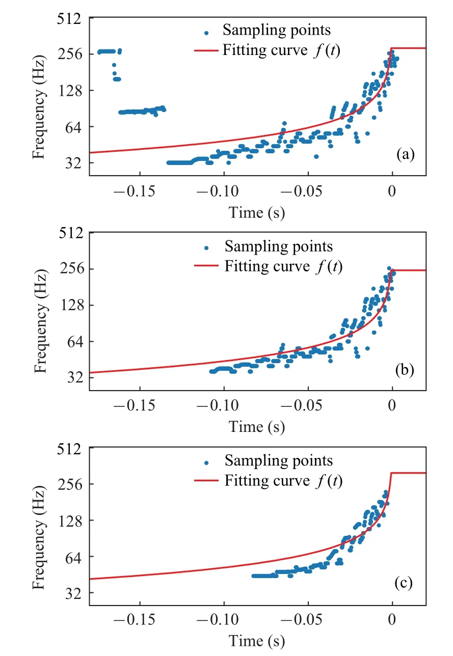
Fig.4.Results of sampling and fitting using different values of k for GW150914 (H1) after matched filtering in Fig.3: (a) k =0.25, ℳfit =24.8 M⊙; (b) k = 0.35, ℳfit = 28.56 M⊙; and (c) k = 0.65, ℳfit =21.98 M⊙.The absolute errors of those results are 4.11 M⊙,0.04 M⊙,and 6.62 M⊙respectively.
Different values ofkwill have different effects on the final estimated chirp masses,resulting in different errors.It can be seen from Fig.5 that ifkis too large or too small,the errors of the final results will increase.This is because the frequency curve can not be directly fitted with the time–frequency spectrogram,so it is necessary to select the relatively strong part of the spectrogram by sampling points for data fitting to estimate the parameters.Ifkis too small, too many sampling points are selected and the noise becomes relatively louder, so the GW signal is easily drowned in the background noise, yielding the data-fitting results unsatisfactory.Ifkis too large and the sampling points are selected too few, the effective points of the signal are relatively reduced and the overall information is reduced, which is also not conducive to data fitting.Only through the appropriatekwe can remove the background noise of the time–frequency spectrogram as much as possible and obtain a better result.
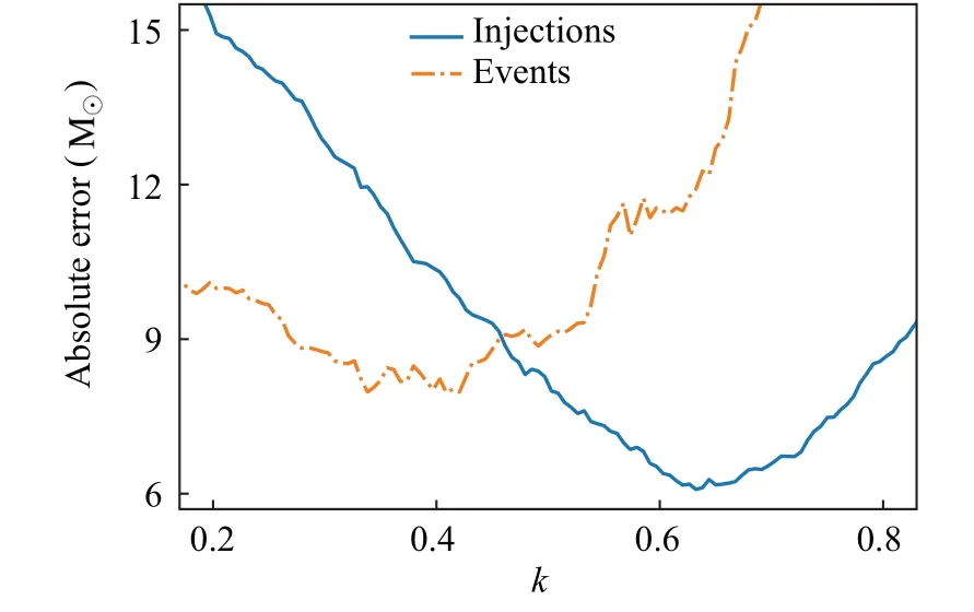
Fig.5.The absolute error of the final results obtained varies with k for injections and events.The error of the injections is the difference between the final results and the parameters of the injected signals, and the error of the events is the difference between the final results and the GWOSC results.
Generally speaking, the more complex the noise is, the smaller the optimalkvalue is,and the greater the error is.But we have not yet found the accurate relationship between the optimalkand the data, so we can only select differentkfor comparison.From Fig.5, it can be found that the optimal value ofkshould be 0.62 for the injections and 0.41 for the events.And we setkfrom 0.4–0.8 for the injections in Subsection 4.2 and 0.2–0.6 for the events in Subsection 4.3.
4.2.Error analysis of injections
One method of verifying a model is to construct simulated signals with accurate parameters to test the model.Through the GW Toolbox web application,we set detector to advanced LIGO(in O3a)and SNR-threshold to 8 for 10 years detection.[52]There are nearly 550 BBH events detected in the simulation.We use SEOBNRv4opt here to generate the BBH signals with the parameters given by GW Toolbox.[53]To generate a frame of simulated O3 Gaussian noise,we use the theoretical PSD (aLIGOaLIGO140MpcT1800545) provided by PyCBC.[41]The frequency of simulated noise ranges from 5 Hz to 4096 Hz.Through the above methods, we have obtained 500 BBH events recorded in fragments with a sampling rate of 4096 Hz in 32 s, including GW signals of 5 s.Next,we use the processing flow in Subsection 4.1 to process and analyze the error of these BBH injections.
The time error and absolute error of 500 injections after processing are shown in Fig.6.From Figs.6(a) and 6(b), it can be seen the time error is extremely small and nearly 97.8%events have time errors within 0.02 s,which is sufficient for the next step of fitting.Events with significant errors are generally low SNR and low chirp mass.As the chirp mass increases,the time error tends to increase.The matched filtering in the merger would lead to a non-physical switch of phase, which might lead to the bias in the estimation.Nearly 2.2% events have time errors greater than 0.02 s because of the phase.
Figures 6(c)and 6(d)reveal the distribution of the absolute errors in relation to the chirp mass and SNR of injections respectively.In the range of chirp mass 5–40M⊙, the estimated chirp mass is ideal, because the low chirp mass ones have higher frequency during the merger phase and the high chirp mass ones have lower frequency,which are filtered during the filtering processing.In the range of SNR 8–48, the estimated chirp mass is ideal,because the low SNR makes the weak signal that makes noise strong.In general, the effect of using this flow to process and analyze the injections is relatively ideal, with the average time error of 0.004 s and the average absolute error of 5.84M⊙.
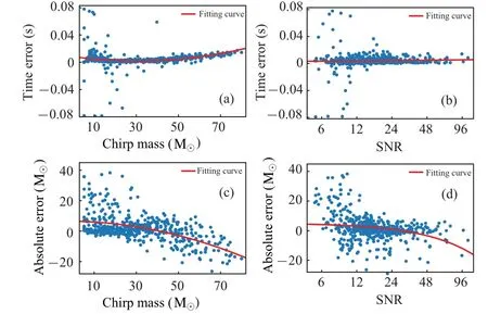
Fig.6.Error analysis for the final results of 500 injections with k=0.4–0.8.Top: analyzing the error of the coalescence time: (a) time error and chirp mass,(b)time error and SNR.The average time error is 0.004 s.The dots in these figures are the means of the results obtained using different k.The fitting curve equations used in Figs.6 and 7 are F(x)=ax2+bx+c.Bottom: analyzing the error between the final results and the parameters of injected signals: (c) absolute error and chirp mass, (d) absolute error and SNR.The average absolute error of the final results is 5.84 M⊙.The average chirp mass of injections is 30.75 M⊙and the average chirp mass of the final results is 32.42+4.61-4.61 M⊙.
4.3.Error analysis of events
From the first detection GW150914 in 2015 to the present day,nearly 100 GW events have been detected and confirmed.The first observing run (O1), the second observing run (O2),and the third observing run(O3)have been completed,and all detected GW events and their details have been published in different catalogs.The Gravitational Wave Transient Catalog(GWTC) used in this paper is from the GWOSC,[54]which contains detected GW events from different detectors,including GWTC-1,GWTC-2,GWTC-2.1,and GWTC-3.[55–58]We select 85 events containing BBH from GWTC for analysis and study the influence of differentk,chirp mass and SNR on the final result.
In Table 2,the results are obtained by processing H1 and L1 withk=0.2–0.6 respectively.The average chirp mass of H1&L1,which take the average of both detectors,are closer to those of GWOSC than those of a single detector.That reveals the feasibility of using the processing method in this paper.
Apart fromk, we consider the effects of chirp mass and SNR on the errors.From Fig.7, it can be seen that around the chirp mass~24.2M⊙, the absolute error is minimum.That is because GW150914 (ℳ=26.8M⊙) is used to adjust the parameters in our NA waveform.Therefore,when the chirp mass is away from 24.2M⊙,the absolute error becomes larger.On the other hand, since the relationship between the SNR and the waveform is complex,we just find a testing result that shows the minimum error appears at SNR~14.4.The error will be enhanced while the SNR is away from 14.4.And Figure 7(c)illuminates that the chirp masses of 72.6%events given by GWOSC are in the confidence interval of 2σgiven by our NA model.That shows that most chirp masses of the BBH GW events can be included in the error distribution of our estimation.
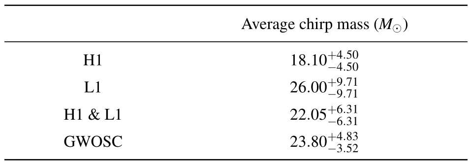
Table 2.The average chirp mass for 85 BBH events.The superscript and subscript represent a standard deviation.H1 and L1 refer to the average chirp mass obtained by processing and analyzing the data of two detectors respectively.H1 & L1 refer to the average chirp mass obtained by considering the analysis results of two detectors’ data at the same time and taking the average value of both as the final result.GWOSC is the average chirp mass calculated according to the values released by GWOSC.
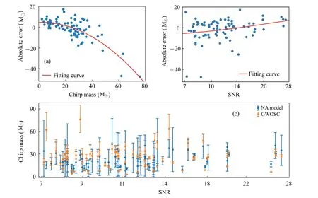
Fig.7.Error analysis for the final results of 85 BBH events with k=0.2–0.6.Top: analyzing the error between the final results and the parameters given by GWOSC:(a)absolute error and chirp mass, (b)absolute error and SNR.These figures characterize the distribution of the absolute errors in relation to the chirp mass and SNR respectively,where the chirp mass and SNR in the horizontal coordinates are given by GWOSC.The dots in these figures are the means of the results obtained using different k.Bottom: (c)SNR and chirp mass with error bar.The yellow dots represent the parameters given by GWOSC.The blue dots are the mean values of our results,and the error bar is the confidence interval of 2σ.There are 72.6%BBH events released by GWOSC in the ranges of error bars from the NA model.
5.Conclusion and prospection
The 20 Hz–1 kHz frequency GWs generated by CBC are significant objects of study for ground-based detectors,and the application of detected data is an essential basis for further research about the parameter estimation and evolution of compact binary systems.We estimate the chirp mass by constructing the NA model adapted to CBC,preprocessing the detected data using data whitening and wavelet transform,determining the GW coalescence time and initial chirp mass using the analytic waveform based on matched filtering,and then estimating the chirp mass by fitting the frequency curve and the sampling points in the time-frequency spectrogram.The above operations constitute the basic process from raw data processing to parameter estimation for BBH.This process allows the parameter estimation of chirp mass in a short time,making good use of the parsimony of the NA model and reducing the shortcomings caused by its low-order approximation.As a simple approximation, the processing and analysis are still feasible and have some reference significance for the data processing of LIGO GW data and parameter estimation of compact binary systems.
Regarding the BNS events, the results obtained through the processing mentioned above are non-ideal.We have simulated BNS injections before when simulating BBH injections, but the results were so unsatisfactory, with absolute error of around 40M⊙.Firstly,that might be because the BNS,whose mechanism is more complicated compared to the BBH,is not well fitted with the NA model, so the accuracy decreases.Secondly,the wavelet used here to convert the whiten data to the time–frequency spectrogram is the Morlet wavelet,while LIGO uses the sine-Gaussian wavelet.[59,60]In the signal processing of the BNS events,the result of Morlet wavelet processing is not very satisfactory, and the signal is almost drowned in the background noise.Finally, the chirp mass of BNS is quite small, making the frequency in the merger and ringdown phases extremely high,even exceeding the Nyquist frequency 2048 Hz.And there is a filtering operation in the processing flow, which filters the parts above 600 Hz.If we raise this threshold, it will result in excessive noise for other events and increase the error.Therefore, the process used in this paper still basically only applies to the case of BBH.
In the future, we will do further research to improve the processing flow of this paper.The NA model is further optimized in terms of theoretical templates to better fit BNS and massive BBH,and to be more realistic in determining GW coalescence time and in fitting the data.The use of more accurate wavelets in data preprocessing makes the GW signal more visible relative to the noise background.In terms of parameter estimation, some improved sampling methods and fitting methods are used to make the information fitted to the data more accurate and the results more consistent with the actual situation.By improving the above aspects,it should be possible to further reduce the errors.
Acknowledgements
Project supported by the National Key Research and Development Program of China(Grant No.2021YFC2203004),the National Natural Science Foundation of China (Grant No.12147102),and the Sichuan Youth Science and Technology Innovation Research Team(Grant No.21CXTD0038).

- Chinese Physics B的其它文章
- Dynamic responses of an energy harvesting system based on piezoelectric and electromagnetic mechanisms under colored noise
- Intervention against information diffusion in static and temporal coupling networks
- Turing pattern selection for a plant–wrack model with cross-diffusion
- Quantum correlation enhanced bound of the information exclusion principle
- Floquet dynamical quantum phase transitions in transverse XY spin chains under periodic kickings
- Generalized uncertainty principle from long-range kernel effects:The case of the Hawking black hole temperature