On the calibration of a shear stress criterion for rock joints to represent the full stress-strain profile

Akram Deiminiat,Jonathan D.Aubertin,Yannic Ethier

Department of Construction Engineering,École de Technologie Supérieure (ÉTS),Montréal,Canada

Keywords:Full shear profile Post-peak shear behavior Rock joint Joint roughness coefficient (JRC)Axial stress-strain curve

ABSTRACT Conventional numerical solutions developed to describe the geomechanical behavior of rock interfaces subjected to differential load emphasize peak and residual shear strengths.The detailed analysis of preand post-peak shear stress-displacement behavior is central to various time-dependent and dynamic rock mechanic problems such as rockbursts and structural instabilities in highly stressed conditions.The complete stress-displacement surface(CSDS) model was developed to describe analytically the pre-and post-peak behavior of rock interfaces under differential loads.Original formulations of the CSDS model required extensive curve-fitting iterations which limited its practical applicability and transparent integration into engineering tools.The present work proposes modifications to the CSDS model aimed at developing a comprehensive and modern calibration protocol to describe the complete shear stressdisplacement behavior of rock interfaces under differential loads.The proposed update to the CSDS model incorporates the concept of mobilized shear strength to enhance the post-peak formulations.Barton’s concepts of joint roughness coefficient (JRC) and joint compressive strength (JCS) are incorporated to facilitate empirical estimations for peak shear stress and normal closure relations.Triaxial/uniaxial compression test and direct shear test results are used to validate the updated model and exemplify the proposed calibration method.The results illustrate that the revised model successfully predicts the post-peak and complete axial stress-strain and shear stress-displacement curves for rock joints.

1.Introduction

Rock masses present networks of structural fractures (i.e.discontinuities and joints) which separate intact rock components.The mechanical properties of these interfaces greatly influence the behavior of rock masses.The potential for failure or rupture of the rock masses (e.g.slope failure,strain burst,rock falls) is largely attributed to shear strength of joint surfaces under load (Ladanyi and Archambault,1969;Barton,1982;Lee et al.,1990).A proper understanding of the shear behavior of structural interfaces is thus necessary to ensure safe and stable rock excavations.

Numerous criteria have been proposed to quantify shear strength of rock joints subjected to lateral and normal loads (e.g.Patton,1966;Bandis et al.,1981;Saeb and Amadei,1992;Grasselli and Egger,2003;Barton,2013;Zhang et al.,2014;Thirukumaran and Indraratna,2016).These models predict the peak and/or residual shear strength of rock fractures based on superficial geometry(i.e.directional roughness)and rock geomechanical properties(e.g.compressive strength,elastic modulus) (Goodman,1980).Limited considerations have been given to the practical quantification of total shear stress-strain profile of joints under loads.The pre-and post-peak strain profiles of loaded joints is of great importance in dynamic environments prone to time-dependent failure and rockburst events (Martin,1993;Martin and Chandler,1994;Fairhurst and Hudson,1999;Simon,1999;Simon et al.,2003;Khosravi,2016;Khosravi and Simon,2018).There are clear needs for a pragmatic and applicable numerical solution to describe the full shear stress-strain profile pre-and post-peak for rock interfaces under differential load.

Simon (1999) introduced a constitutive model to represent the complete stress displacement surface,the complete stressdisplacement surface (CSDS) model.The model considers strains arising from compaction,shear,and normal deformation and it includes several model parameters that are needed to be obtained by triaxial compression and direct shear test data and extensive curve fitting (Simon,1999;Simon et al.,2003).Subsequent works have been reported to develop and verify the proposed model(Deng et al.,2004;Tremblay,2005;Tremblay et al.,2007;Khosravi,2016).Notwithstanding,difficulties with the estimation of model parameters have never been removed,and the exemplified calibration process for CSDS remains opaque due to extensive curve fitting that diminishes the applicability of the model to practical realities of rock engineering.A rational for intuitive procedural calibration is required to develop CSDS further for holistic applications.

The goal of this work is to present a thorough stepwise procedure for the calibration of a complete shear stress-strain model.To this purpose,a modified version of the CSDS model is proposed to incorporate updated formulations for peak strength and normal closure,and account for mobilized shear strength.Validation for the updated model and the proposed calibration protocol is exemplified with experimental data taken from relevant literature.The results showcase the applicability of the model to represent the stress-strain behavior of rock interfaces during conventional direct shear and triaxial shear tests.This paper contributes a complete and readily applicable version of the CSDS model not published before,introduces an update to the model to reflect modern acknowledged precepts of field,presents a detailed and exhaustive calibration procedure to determine model parameters,showcases a multi-datasets validation of the model to showcase its applicability and the proposed calibration protocol,and demonstrates a number of application methods based on different shear testing programs(with direct and/or triaxial testing for post-peak and full profile representation).

2.Background

The shear behavior of rock interfaces can be characterized through direct or indirect experimental methods in laboratory settings.Direct shear testing and shear characterization in triaxial apparatus are described in ISRM (1989),ASTM D2664-04 (2004),ASTM D5607-16(2016),ASTM D7012-23(2023),(see also Franklin et al.,1974;Fardin,2008;Tang and Wong,2016;Liu et al.,2017;Day et al.,2017a,b;Packulak et al.,2018,2022a,b).Fig.1 depicts conceptually the stress-strain profile for a rock joint under shear loading.Similar features and profiles are expected from applying compression to a sample during direct shear and triaxial compression tests.The plot is characterized by near linear stressstrain correlation up to a maximum stress value associated with peak shear stress.Peak shear stress denotes the shearing and or crushing of superficial asperities,thus changing the roughness and potential for dilation.The post-peak behavior of rocks starts once the failure plane is created and the shear load decreases,eventually converging to a constant value and coined residual stress(Goodman et al.,1968;Goodman,1976;Barton and Choubey,1977;Martin and Chandler,1994;Aubertin et al.,1998;Eberhardt et al.,1998).

Fig.1.Typical shear stress versus deformation curve for a rock joint under shear loading.

Joint deformation under normal load is quantified by its normal stiffness,Kn(MPa/mm)(Goodman et al.,1968).It can be measured by varying normal stress and measuring the corresponding strain normal to the discontinuity.The relation of normal stiffness with peak and residual shear displacement and maximum joint closure allows one to identify the contribution of joints to total displacement of a rock mass (Fotoohi,1993).Joint shear behavior is highly affected by the change in normal stress (Goodman et al.,1968;Bandis,1980;Fotoohi,1993;Simon,1999).

The shear behavior of rock joints is heavily dependent upon external factors (e.g.shear load direction,span,stress profile) and the geomechanical characteristics of the rock and its interfaces(e.g.morphology of discontinuities,mechanical strength,elastic properties,weathering conditions).Extensive studies have parametrized the influence of intrinsic and external factors on the behavior of rock joints under differential loads (see for example Goodman et al.,1968;Barton,1973;Bandis,1980;Simon,1999;Grasselli,2001;Fardin et al.,2001,2004;Simon et al.,2003;Fardin,2008;Sanei et al.,2015a;Tang and Wong,2016;Khosravi,2016;Yang et al.,2016;Liu et al.,2017;Niktabar et al.,2017;Li et al.,2022;Wang et al.,2022).

Various criteria have been proposed over the years to quantify peak shear strength of rock joints with respect to the applied normal load by accounting for both external and intrinsic factors.Patton (1966) proposed a bilinear model by incorporating surface roughness (i.e.asperities) to Mohr-coulomb failure criterion.Ladanyi and Archambault(1969)developed a more comprehensive failure model,the LADAR model,based on actual shear contact surfaces and inclination angle,and applicable to different irregular joint surfaces.Since then,several failure criteria have been developed by implementing roughness parametrization (e.g.Barton,1973;Barton and Choubey,1977;Bandis et al.,1981;Barton,1982;Fortin et al.,1988;Amadei and Saeb,1990;Saeb and Amadei,1992;Huang et al.,1993;Haberfield and Johnston,1994;Homand et al.,2001).

The joint roughness coefficient (JRC) proposed by Barton and Choubey (1977) progressively became a standard index of reference to represent joint surface geometry (ISRM,1978).The subjective nature of this index has been discussed at length by various authors(Grasselli,2001;Sanei et al.,2015b;Khosravi,2016;Li et al.,2022).Researchers proposed correlations between objective roughness parameters(e.g.fractal dimension,D;roughness profile index,Rp;surface parameter,Z2) andJRC(Yang et al.,2001;Jang et al.,2006;Kim et al.,2009;Tatone and Grasselli,2010).Grasselli(2001) used apparent dip angle of joint surface with respect to the shear direction to find a three-dimensional (3D) criterion for the estimation of peak shear strength of the entire rock joint surface.This method was followed by many researchers (Grasselli et al.,2002;Grasselli and Egger,2003;Xia et al.,2014;Tang and Wong,2016;Yang et al.,2016;Liu et al.,2017;Tian et al.,2018;Magsipoc et al.,2020).

Models based on mobilized shear strength have also been proposed to predict the post-peak shear strength (e.g.Bandis et al.,1983;Asadollahi,2009).Simon (1999) developed the CSDS model to describe the post-peak shear behavior for rock joints in the context of describing rockburst-prone rock mass conditions.Themodel was refined and adapted to predict the hydromechanical behavior of rock joints by Tremblay et al.(2007).

The present study aims to adapt the CSDS model by incorporating peak shear strength,mobilized joint roughness and normal closure models.In addition to provide a simple procedural method for calibration,the adapted model can describe full shear behavior of rocks from triaxial/axial compression tests with or without direct shear tests.In this article,the CSDS model is first introduced.Certain and proven formulae that are used to modify the models’calibration method are presented next.The step-by-step CSDS model calibration proposed in this study is then presented and exemplified by using a series of data sets taken from the literature.

3.Complete stress displacement surface (CSDS) model

The CSDS model implements an exponential function to describe the relationship between shear stress τ (MPa) and shear displacementu(mm) (Simon,1999):

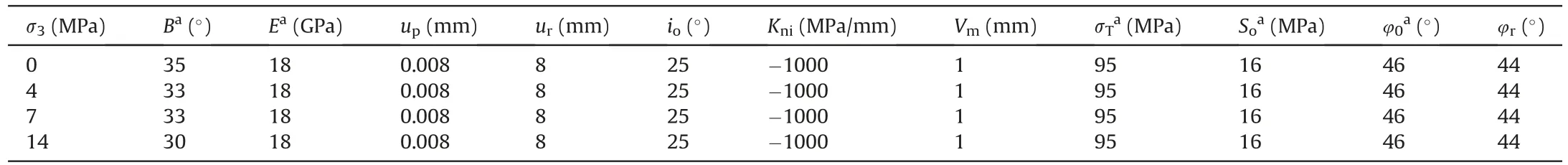
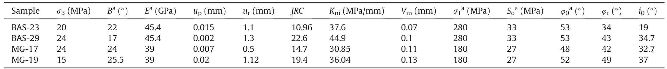
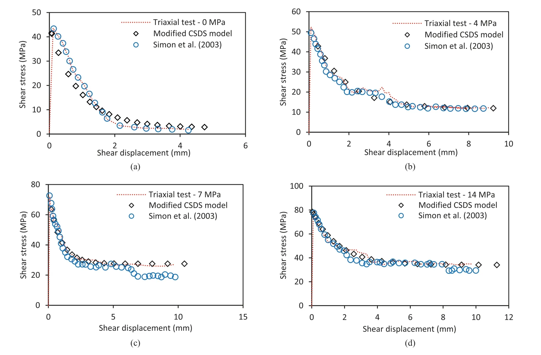
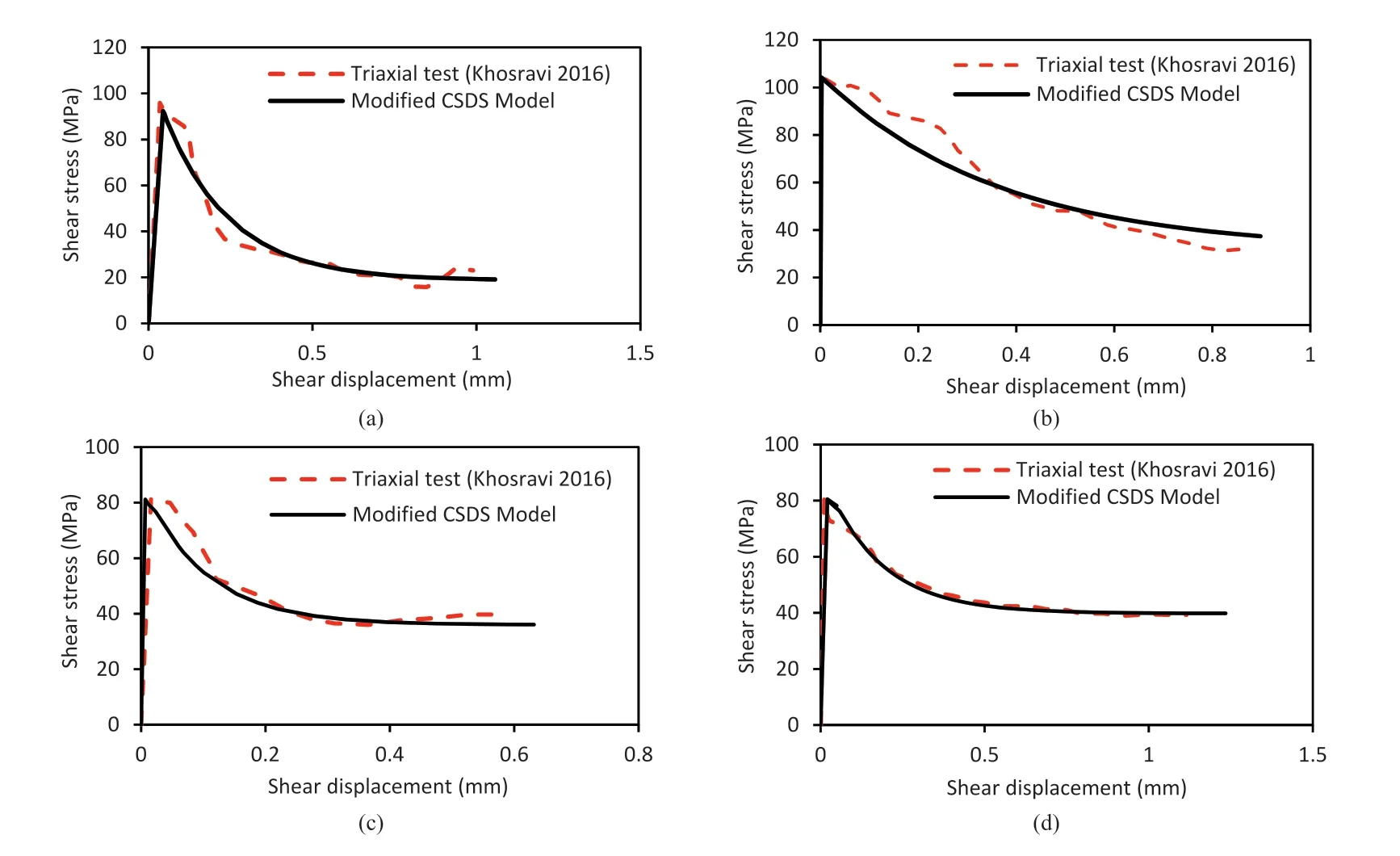
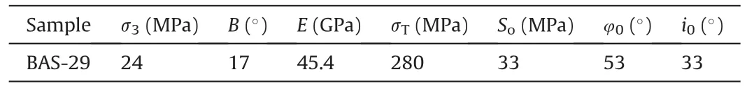
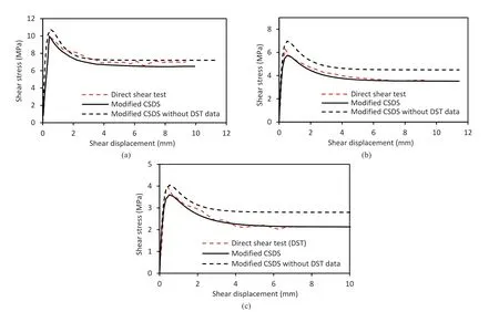
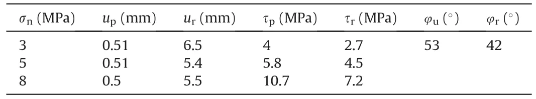
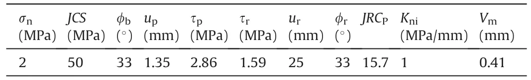
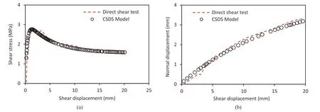
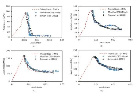
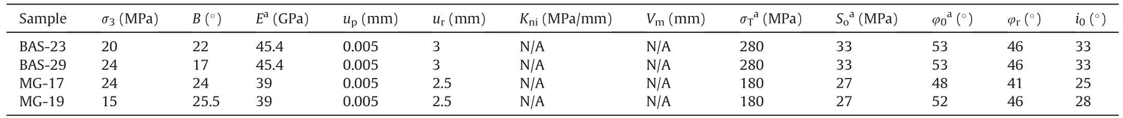
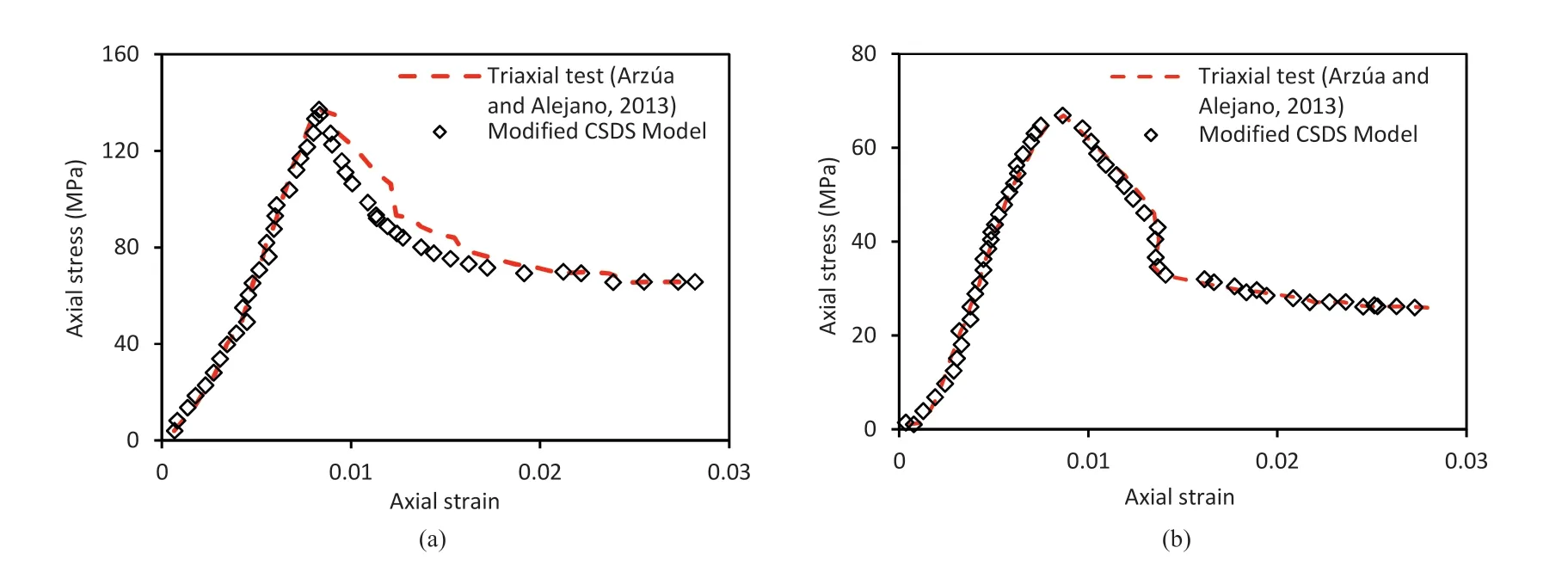
wherea,b,c,dandeare the model parameters with the condition ofa,b,c,d,e>0 andc

Boundary conditions for the model formulation help derive values of model parameters.Under initial testing conditions (i.e.u=0),there is no deformation and no corresponding load.Therefore,we have

At large displacement(i.e.u≫0),it is intuited that shear stress has reached residual state τr(MPa).The two exponential components approach 0,thus we have

When shear deformation has reached residual conditions (i.e.u=ur),then it follows that

Then,we have

Based on extensive experimental data,Simon et al.(2003)proposed to approximate exponential component of -curas 0.07,i.e.

Since shear stress peaks atu=up,the derivative of Eq.(1) withu=upmust equal zero,i.e.

At peak displacement,F(up)=τp,thus we have

Parameterdis isolated in Eq.(10) to yield

where τpand τrare the peak and residual strengths,respectively(MPa);andupandurare the displacements at the peak and residual shear stresses,respectively(mm).

Based on Eqs.(2)-(11),the model parameters can be derived from physical measurements obtained in the conventional laboratory experiments.

An exponential function was proposed by Simon (1999) to describe the normal displacement (V) versus shear displacement(u) relationship:

where β1,β2and β3are the model parameters.The procedure for determining these parameters is described below.

It goes from the above equation that foru=0,V≡β1-β2.β2is derived by following the relationship between normal load and displacement described by Bandis et al.(1983):

where σnis the normal stress applied to rock joint(MPa),Vmis the maximum closure of the rock joint (mm),andkniis the initial normal stiffness (MPa/mm).It follows that

Atu≫0,V=β1andu=ur.

By using the model proposed by Goodman and St John (1977)(Eq.(15)),one can obtain β1using Eq.(16).

Sunrise on the eastern coast is a special event. I stood at Dolphin s Nose, a spur jutting1 out into the Bay of Bengal, to behold2 the breaking of the sun s upper limb over the horizon of the sea. As the eastern sky started unfolding like the crimson3 petals4 of a gigantic flower, I was overcome by a wave of romantic feelings and nostalgia5（，） -- vivid memorie not diminished by the fact that almost ten years had passed.

where σcis the compressive strength of rock(MPa),k2=4,andi0is the initial asperity angle (°).

Based on many experimental data taken by Simon (1999) from the literature,it was found that the last parameter,β3,may be related to the residual displacement (ur) as follows:

4.Proposed modification to the CSDS model

A series of modifications is proposed to improve CSDS’ ease of calibration.These changes provide specific and proven formulations for certain model parameters that may otherwise require extensive curve fitting.The modifications and rationale for empirical justifications are described below.A compiled summary of the updated CSDS formulation is provided in Table 1.

Table 1Summary of the updated CSDS formulation.

4.1.Normal closure model after Bandis et al.(1983)

Rock joint deformability can be described by the properties of stress-deformation curve (Goodman et al.,1968;Fotoohi,1993).Exponential equations have been suggested by Bandis et al.(1983)to determine the maximum closure and initial normal stiffness as follows:

whereajis the initial joint aperture(mm)and it can be obtained by

where σcis the uniaxial compressive strength(MPa)andJCSis the joint compressive strength (MPa).Eqs.(18)-(20) are proposed to facilitate the determination of β1and β2in Eqs.(14) and (16).

4.2.Mobilized shear strength after Barton (1982) and Asadollahi(2009)

Barton (1982) modified the peak shear strength model of Barton-Bandis to take the stress dependency of shear strength into account.The modified model considers the progressive degradation of joint roughness during the shear process,mobilized joint roughness coefficient(JRCm).The failure model is then proposed as follows:

where τ is the mobilized shear stress (MPa) and φris the residual friction angle (°).

Asadollahi (2009) modified Barton’s model for the peak displacement and the dimensionless relationship betweenJRCand shear displacement to predict the shear strength more precisely:

whereLis the specimen length (m).

Asadollahi and Tonon (2010) validated proposed models by using 365 direct shear test data taken from the literature in which theJRCranged between 0 and 20 with normal distribution.The average ratio of predictedupover measuredupwas reported as 1.11 with standard deviation of 0.76 and the average ratio of predictedJRCmobilisedto measuredJRCmobilisedwas 1.19 with standard deviation of 0.92.

Furthermore,Fig.2 shows the application of Barton and Asadollahi models for the direct shear tests on a cement mortar with irregular surface,which are taken from Ohnishi et al.(1993).As shown,the post-peak shear stress obtained by Asadollahi (2009)predicts quite well the experimental curve whereas the curve obtained by Barton model decreases as the shear displacement increases.This observation may be due to the 0-value defined in Barton’s table forJRCm/JRCpwhenJRCp>5 andu/up=25.Hence,the model proposed by Asadollahi (2009) is used in this study to determine theJRCmandup.

Fig.2.A comparison between the post-peak shear behavior of rock joint predicted by Barton and Asadollahi models and experimental data obtained by Ohnishi et al.(1993).

Since theJRCmis obtained from Eq.(23)for all the data points on the experimental curve,the CSDS model parameter,β1,is suggested to be calculated as follows:

4.3.Peak shear strength criterion after Barton and Choubey (1977)

Barton and Choubey (1977) proposed the commonly acknowledged peak shear strength criterion based on roughness conditions(represented byJRC) and joint compressive strengthJCS:

JRCpcan be obtained directly by profiling rock joint specimens using profilometer.Ten typical roughness profiles given by Barton(1973) forJRCranging from 0 to 20 can then be used.The joint roughness coefficient can also be determined by the backcalculation of Eq.(26),when other parameters are available from the experimental data.In this equation,JCScan be determined by Schmidt hammer tests.Alternatively,JCScan be estimated as the unconfined compressive strength (σc) of the intact rock for fresh joints and σc/4 for highly weathered rocks (Barton,1973;Barton and Choubey,1977).Additional information onJCSmeasurements,empirical estimates and complementary techniques for the application ofJRCandJCScan be found in Barton(2013),Zheng and Qi (2016),Liu et al.(2017),and Tang et al.(2021).For further analyses in this work,the peak value of shear strength predicted from Eq.(1)and/or measured by experimental work is considered equal to the peak shear strength obtained by Eq.(26).The Barton model is suggested here because of easy application of the model in industry and general trust in the calculations based onJRCandJCS.

5.CSDS model calibration

This section describes the updated calibration method of CSDS model for post-peak and full shear behavior of rock discontinuities with the use of triaxial compression test with/without direct shear test data.The model calibration includes some general steps remained from Simon et al.(2003) and detailed steps proposed in this study.The model is then exemplified in the next section.

5.1.Post-peak shear stress-displacement curves with triaxial/uniaxial compression tests

The CSDS model can be applied to describe traditional direct shear testing detailed by ISRM (1978)and ASTM D5607-16(2016).As reported by Simon et al.(2003),the relevant experimental parameters,i.e.φb,τp,τr,up,ur,JCSand elastic modulus (E) are first obtained from traditional interpretation of triaxial and uniaxial testing experimental process.Then,the model parameters such asa,b,c,dandeare determined through Eqs.(2)-(11).The following procedural workflow,proposed in this study,is subsequently used to calibrate the model.

(1)JRCpis obtained by back calculation from Eq.(26).

(2) For all the post-peak data points on triaxial stress-strain curve,the ratios ofu/up(or ε/εp) are calculated and added to Eq.(23) to determineJRCm.

(3) Values foraj,VmandKniare directly calculated by Eqs.(18)-(20) to ensure that the influence of joint deformation is considered in the analyses.

(4) By using the obtained parameters and experimental data,the CSDS model parameters β1,β2and β3can be determined through Eqs.(14),(17) and (25),respectively.

(5) The variation of axial strain on the post-peak stress-strain curve is a function of several parameters(Simon et al.,2003):

where ε is the axial strain,εpis the peak strain,Δuis the difference in shear displacement (mm),ΔVis the difference in normal displacement (mm),Δσ1is the difference in principal axial stress(MPa),Lis the initial sample length(mm),Eis the elastic modulus of rock (MPa),and β is the shear plane angle (°).

For each data on the post-peak stress-strain curve,the peak and elastic strains are subtracted from Eq.(27),thus we have

where ε*is the modified post-peak strain.

At the 1st point,ΔV1=V1=0.Eq.(27) becomes

At the 2nd point,from Eq.(12),we have

From Eq.(27),we have

The same procedure is repeated for all subsequent datapoints on the post-peak stress-strain curve.The calculated values of Δuand model parameters are used in Eq.(1)to determine the shear stress.

5.2.Full shear stress-displacement curves with triaxial compression tests,with/without direct shear tests

When direct shear tests are available,the model properties(e.g.τp,τr,up,ur)are directly derived through the shear curves in order to determine the model parameters such asa,b,c,dande.Once the model parameters are determined,Steps (1)-(5) in the preceding section are carried out by using the axial stress and strains obtained from triaxial compression tests.It should be noted that,since the complete shear displacement is required in this section,the values ofuobtained by following Step(5)are used in Eq.(1)for estimating the shear stress.

An alternative method is proposed in this study to approximate the calibration process in the absence of direct shear test data.In this method,the measured joint roughness coefficient and Barton model can be used to determine peak shear strength (τp).The Coulomb criterion without cohesion is used to obtain the residual friction angle:

The φris thus used to calculate the residual shear strength under the imposed normal load(s).The corresponding residual displacement for τris denoted byurthat can be determined using curve fitting and back calculation of CSDS model.SinceJCSandJRCpare known,Eq.(24)may be utilised to determineup.When direct shear test does not reach the actual residual shear stress and subsequently residual shear displacement,the residual shear data can be obtained by the alternative method.

5.3.Full shear stress-displacement curves with direct shear tests

When the direct shear test data and mechanical properties of rock (e.g.φb,JCS(or σc),E) are available,the model properties are directly extracted from shear curves to determine the model parameters such asa,b,c,dandeusing Eqs.(2)-(11).Subsequently,the shear stress can be calculated.Depending on the direct shear machine and applied normal load,direct shear test may not reach the actual residual shear stress and subsequently residual shear displacement.The residual shear stress can thus be obtained by using Eq.(31),andurcan be back-calculated with the CSDS model(Eq.(1)) and curve fitting.

Concerning the normal displacement-shear displacement curves,the method suggested in this study is followed.The mobilizedJRCvalues are first obtained from Eq.(22).Then,the normal closure parameters (e.g.aj,Vm,Kni) are determined to be able to calculate the model parameters β1,β2and β3and normal displacement from Eqs.((12),(14),(17) and (25).Since the suggested formulae for the estimations of β1and β2are based on normal stress,only one value is obtained for each parameter.

5.4.Full axial stress-strain curves with triaxial/uniaxial compression tests

The proposed method for post-peak stress-strain estimation resembles the method initiated by Simon et al.(2003),with some modifications that are highlighted below along with the proposed method for pre-peak curve.

The model parameters must first be determined from triaxial compression tests using the procedure outlined in Section 5.1.Once the model parameters are obtained,the following steps must be taken:

(1) For the data on stress-strain curve,the shear and normal stresses are calculated by the following formulae:

where σ1is the major principal stress (MPa),and σ3is the minor principal stress(MPa).

(2) For the corresponding values of shear stress,the shear displacement (u) can be computed through Eq.(1) and the application of a linear solver available in common computation tools(e.g.MS Excel solver,see the detailed application in Li et al.(2000)).There are two values foru,which should be noted.The value larger than the peak displacement (up)should be used for the current analysis.

(3) By using the predicteduvalues,obtained β1(by using Eq.(25) suggested in this study),β2and β3and Eq.(12),the normal displacement (V) can be calculated.

(4) The axial strain can then be estimated by adding the predicted shear and normal displacements into Eq.(27).For the pre peak profile,since the volume change is positive before shear stress reaches to the peak(Goodman,1976;Martin and Chandler,1994),the normal displacement should be obtained using Eq.(34).The axial strain can thus be predicted with Eq.(35).

where εpre-peakis the axial strain before peak.

6.Validation of updated CSDS

6.1.Scope of validation work carried

The next sections showcase the use and application of the CSDS model in its updated form,and the calibration method proposed in the previous sections.The model is applied to different experimental settings commonly encountered with laboratory characterization for shear testing.Validation is carried out for test programs with triaxial and/or direct shear tests for post-peak and full profile representations.The validation work was carried out on direct shear and triaxial compression tests originally presented in Price (1979),Ohnishi et al.(1993),Arzúa and Alejano (2013),Khosravi and Simon (2018) and Khosravi (2016).These data sets include both direct and triaxial shear test results with servocontrolled machine for the full pre-and post-peak profile.

6.2.Post-peak shear stress-displacement estimation with triaxial compression tests

This section exemplifies the application of the updated model to describe post-peak shear stress-displacement curve.The curves predicted by the original CSDS model (Simon et al.,2003) are also included in the results to showcase the validity and evolution of the model.The experimental data on sandstone were taken from Price(1979) for different confining pressures.

Table 2 shows the rock properties and CSDS model properties obtained by Simon et al.(2003)for four tests,and Table 3 gives the model properties that are determined by the updated model for different confining pressures.Fig.3 illustrates a comparison of post-peak shear stress-displacement curves obtained by this study and those taken from Simon et al.(2003).The results reveal that the new model always calibrates well the residual shear stress.It is perfectly illustrated in Fig.3c and d.In addition,it is noted from Table 2 that thekniandVmvalues obtained from curve fitting are seemingly arbitrary and/or subjective to the user.The updated method presents a systematic solution to derive these values as showcased in Table 3.

Table 2Rock properties and CSDS model properties that are obtained by Simon et al.(2003).

Table 3Rock properties taken from Price (1979) and the model properties obtained in this study.

Table 4Rock properties taken from Khosravi (2016),and the model properties obtained in this study for basalt (BAS)and microgabbro (MG).

Table 5Rock properties taken from Arzúa and Alejano (2013),and the model properties obtained in this study.

Fig.3.Comparison of the post-peak shear stress-displacement curves obtained by the updated model with those obtained by Simon et al.(2003)for triaxial compression tests on sandstone with confining pressures of (a) 0 MPa,(b) 4 MPa,(c) 7 MPa and (d) 14 MPa.The experimental data are taken from Price (1979).

Fig.4.Post-peak shear stress-displacement curves obtained by the modified model,and the original curves reported by Khosravi(2016)for(a)BAS-23,(b)BAS-29,(c)MG-17,and(d) MG-19.

To further validate the proposed model,the triaxial compression tests on basalt (BAS) and microgabbro (MG) reported by Khosravi(2016) and tests on granitic rock (Blanco Mera) reported by Arzúa and Alejano (2013) are used.Tables 4 and 5 show the rock properties taken from the literature and the model properties obtained in this study for BAS and MG and Blanco Mera,respectively.

Since no representative curves predicted by the original CSDS model could be found in Arzúa and Alejano (2013) and Khosravi(2016),Figs.4 and 5 illustrates a comparison between the original curves reported by these studies and the post-peak shear behavior of the tested rocks obtained in this work.It is shown that the postpeak shear curves of all tests accurately represent the original curves.Similar observation can be made from Fig.5 between the curves obtained in this work and the original curves obtained by Arzúa and Alejano(2013).It is questionable,however,whether the predicted shear stress-displacement curves from triaxial compression testing can also represent the curves obtained from direct shear tests.This issue is addressed in the following section.

Fig.5.A comparison of the post-peak shear stress-displacement curves obtained by the modified model to the original curves reported by Arzúa and Alejano (2013) for (a)σ3=4 MPa and (b) σ3=12 MPa.

6.3.Full shear behavior estimation with triaxial compression tests,with/without direct shear tests

To evaluate the accuracy of the proposed method for the full shear stress-displacement curve,two series of laboratory test results are used.One series are the results of triaxial compression tests on BAS-29 that are reported by Khosravi (2016).Another series are direct shear test data of the same rock obtained by Khosravi and Simon (2018) at normal loads of 3 MPa,5 MPa and 8 MPa.Table 6 shows the rock characteristics used for the analysis.Table 7 shows the direct shear test data from Khosravi and Simon (2018),whereas Table 8 shows the model properties obtained in this study by the updated model.

Table 6Rock properties used in this study.The data are taken from Khosravi (2016).

Table 7Direct shear results of BAS-29 from Khosravi and Simon (2018) at three normal stresses.

Table 8Model properties obtained in this study by the application of the updated CSDS model.

The full shear curves of the tested rock are shown in Fig.6 for different methods at three normal loads.A comparison between the predicted and original curves reveals that the proposed model correctly predicts the pre-and post-peak shear stressdisplacement curves at varying normal loads.The similar conclusion can be given by comparing the model properties presented in Tables 7 and 8 However,significant differences are observed,when comparing theupandurvalues obtained with triaxial compression test data(see Table 4)to those obtained with direct shear test data of the same rock(see Table 8),indicating that direct shear tests are required to obtain reliable full shear stress-displacement curves for a rock joint.

Fig.6.Comparisons between full shear stress-displacement curves obtained by direct shear tests(DST)and those predicted by the modified CSDS model with and without DST.The experimental data are taken from Khosravi and Simon (2018) for normal loads of (a) 8 MPa,(b) 5 MPa and (c) 3 MPa.

The experimental data of BAS-29 are used again to further demonstrate how the full shear curves can be obtained without direct shear test data.In Table 9,one can see the model properties obtained by using the alternative method.

Table 9The model parameters obtained in this study by using the modified CSDS method without direct shear test data.

The full shear stress-displacement curves obtained without the use of direct shear tests are illustrated in Fig.6 for different normal loads.As seen,the curves obtained by applying the normal stresses of 5 MPa and 8 MPa are successfully predicted.However,the predicted post-peak zone in Fig.6c seems to have a difference of 0.5 to the residual shear stresses obtained with the use of direct shear tests.This may be shown further by comparing the data presented in Tables 7-9 for the three normal loads.The model properties in Table 9,which correspond to the predicted curves without direct shear tests,are quite close to those in Tables 7 and 8 These results tend to show that when direct shear tests are not available,the alternative method may be used to describe the full shear stressdisplacement curve.Nevertheless,more works with the use of experimental data of different materials under different normal loads are required to further validate the alternative method.

6.4.Full shear stress-displacement and normal-shear displacement curves estimation with direct shear tests

The accuracy of the proposed method for the full shear stressdisplacement curves when only direct shear tests are available is studied by using the experimental data of cement mortar with irregular surface taken from Ohnishi et al.(1993).Table 10 indicates the characteristics of the rock sample and the CSDS model properties obtained in this study.Fig.7 shows the full shear stressdisplacement and normal-shear displacement curves obtained from direct shear tests and those obtained by the proposed method.The curves obtained in this study exhibit the same trends as those of the original curves.For the experimental data,the shear stressdisplacement curve tends to not behave as a perfect curve.This can be due to the rock joint deformation and rock asperities.

Table 10Rock properties taken from Ohnishi et al.(1993)and the model parameters obtained in this study.

Fig.7.Validation of the model for(a)shear stress-displacement and(b)normal-shear displacement curves of cement mortar with irregular surface.The direct shear test data are taken from Ohnishi et al.(1993).

6.5.Full and post peak axial stress-strain curves estimation with triaxial compression tests

The triaxial compression test results of sandstone reported by Price (1979) are used to obtain the post peak axial stress-strain curves using the updated CSDS model.The rock properties taken from Price (1979),the model properties obtained by the original CSDS model and those obtained by the updated CSDS model in this study are previously reported in Tables 2 and 3,respectively.

Fig.8 compares the experimental post peak stress-strain curves and those obtained by Simon et al.(2003) and this study.As seen,the updated model always results in curves that perfectly fit the original curves.The curves obtained by the original model do not show the residual stress.In all the curves,the post peak stress decreases when the axial strain increases.Unlike,the predicted curves in this study show the same trend as those of experimental data.This observation may be explained by including the mobilizedroughness and joint normal closure model into the analyses after peak.

Fig.8.Comparisons between the post-peak axial stress-strain curves obtained by this study and Simon et al.(2003) with the experimental curves taken from Price (1979) for confining pressures of (a) 0 MPa,(b) 4 MPa,(c) 7 MPa,and (d) 14 MPa.

The full axial stress-strain curves can also be described by the updated model for rock joints.To this purpose,the triaxial compression tests on BAS and MG rocks reported by Khosravi(2016) are used.The model properties obtained in this study for BAS and MG are presented in Table 4.Table 11 shows the rock properties and model properties obtained by Khosravi(2016)using the original CSDS model.According to the data in Table 11,similar peak displacement equal to 0.005 mm was obtained for different samples and different confining pressures.The influences of confining pressure and rock properties on the peak and residual displacements are ignored in the method used by the authors.Furthermore,the values ofkniandVmare not published,and it is unclear how the normal displacement parameters are obtained by the CSDS model.

Table 11Rock properties and CSDS model properties obtained by Khosravi (2016) for basalt (BAS)and microgabbro (MG).

Fig.9 illustrates the experimental and predicted full stressstrain curves for different rocks.Comparisons of the original curves with the curves obtained by Khosravi(2016)and this study show that the updated model provides more accurate results for the full stress curves of four rocks,notably for the post-peak zone and residual stress.

Fig.9.Comparisons of full axial stress-strain curves obtained by this study and Khosravi(2016)for(a)BAS-23,(b)BAS-29,(c)MG-17,and(d)MG-19 with the experimental curves taken from Khosravi (2016).

Similarly,the triaxial compression test results of granitic rock,Blanco Mera,reported by Arzúa and Alejano (2013) are used to further evaluate the updated model.The rock joint properties taken from literature as well as the model properties obtained in this study are presented in Table 12.Fig.10 compares the predicted full stress-strain curves with the original curves for confining pressures of (a) 4 MPa and (b) 12 MPa.The complete profiles between axial stress and strain precisely fit the experimental curves.These results confirm once again the validity of the proposed model.

Table 12Rock properties taken from Arzúa and Alejano (2013),and model properties obtained in this study.

Fig.10.Comparison of the full stress-strain curves obtained by the modified model with the experimental curves reported by Arzúa and Alejano(2013)for(a)σ3=4 MPa and(b)σ3=12 MPa.

7.Discussion

The present work aimed to contribute the field of rock engineering with a complete shear stress-displacement model developed for holistic applications and with a comprehensive calibration method.To achieve this development,an updated version of the CSDS model was presented to address certain practical limitations of the original formulations.The proposed model considers direct estimation of normal closure parameters (e.g.VmandKni) and implements mobilized joint roughness coefficient for peak and residual approximations.A procedural step-by-step protocol was presented to guide calibration efforts using laboratory experiment data from direct shear tests and triaxial shear tests.

Validations carried on various experimental data sets demonstrate that the suggested method improved the calibration of the CSDS model for the post-peak and full shear behavior of rock joints.Additional work shall be carried in the future to further validate the application of the model to other data sets,other types of rocks,and other testing configurations.Deng et al.(2006) presented an application of the original CSDS model to different types of interfaces with infills.Validation of the updated model should be carried out to showcase the applicability of the model to varying types of interfaces,and also address conditions of interests such as rock-concrete interfaces (see also work by Renaud et al.(2019)).

The model currently presents limitation in regards to its numerical formulation which cannot be readily implemented in anumerical code.Future work shall be conducted to adapt the model formulation as a set of partial differential equations (PDE) considering computing cycles/steps.In its current form,the model does not account for strain rate or loading rate,which would leave unknown elements to a complete PDE formulation of the model.Simon (1999) proposed an incremental version of the original model for numerical applications which incorporated assumptions pertaining to the range of displacement rates applicable to the model.Further investigation and laboratory tests should be carried out to refine this aspect and clarify the relationship between strain rate and model response.

Despite advantage of the modified model in incorporating mobilized roughness into the updated method for the predictions of shear stress and normal displacement,the scale effect on this factor was not considered.It is generally acknowledged that the shear behavior and deformability of rock joints are affected by scale.Numerous researchers(e.g.Miller,1965;Pratt,1974;Rengers,1970;Barton and Choubey,1977;Bandis et al.,1981;Yoshinaka et al.,1993;Ohnishi et al.,1993;Fardin,2008;Bahaaddini,2017;Tan et al.,2019;Deiminiat et al.,2022) have investigated the scale effect on the peak shear stress.Meanwhile,Deng and his colleagues studied the scale effect on the post-peak shear behavior of rock joints for the first time in 2004.They investigated the impact of scale on joint behavior based on the measurement of initial asperity angle of joint surfaces in the CSDS model,whereas the mobilized roughness upon shearing of joints of different lengths appear to be responsible for the scale effect in rock joints (Bandis,1990).Since the CSDS model uses the initial asperity angle in calculations of shear behavior and normal displacement,it does not take into account the influence of scale on ongoing deformation during shear and after peak.

However,incorporating the mobilizingJRCand Barton model into the updated model is intended to pave the way for topographical measurements(e.g.LiDAR scanners)and post-processing calibration of the model.Remote sensing topographical data of natural rock joints may be used to find a correlation between the roughness properties of small and natural rock joints.Select researchers have developed peak shear strength models that directly correlate peak shear strength to rock joint properties in a 3D effective area (e.g.Grasselli and Egger,2003;Tatone and Grasselli,2010;Tang and Wong,2016;Yang et al.,2016;Liu et al.,2017;Magsipoc et al.,2020;Huang et al.,2022).Due to the requirement of these models for direct measurement of change in roughness with respect to shear plane direction,they have not been considered in this work.Instead,Barton model is used so that scale-free roughness could be easily included into prediction of shear strength and normal displacement in future works.Using the scale-dependent roughness coefficient in the estimation of shear behavior offers a novel opportunity to describe the post-peak and full shear behavior of large rock joints without scale effect using the updated CSDS model.

8.Conclusions

The following conclusions and observations are drawn from this work and results presented:

(1) It is crucial to consider the mobilized joint roughness coefficient (JRCm) in the estimation of post-peak shear behavior.It could also be seen from the comparison shown in Fig.2.

(2) The updated model well describes the post-peak and complete axial stress-strain curves with the use of triaxial compression test data.

(3) Available and updated versions of CSDS model could predict the post-peak shear stress-displacement curves with the use of triaxial compression test results.These curves,however,do not correspond to those obtained by direct shear test results.

(4) The updated model accurately obtains the complete shear stress-displacement curves.A requirement for making accurate prediction is to use direct shear test data for the estimate of model parametersa,b,c,dande.

(5) In the absence of direct shear test data,the alternative method proposed in this work may be used to determine model properties for the prediction of full shear stressdisplacement profiles.Nevertheless,more works on the validation of this method can be necessary with using the experimental data of different materials obtained under different normal loads.

Declaration of competing interest

The authors declare that they have no known competing financial interests or personal relationships that could have appeared to influence the work reported in this paper.

Acknowledgments

The authors acknowledge the financial support from Natural Sciences and Engineering Research Council of Canada through its Discovery Grant program (RGPIN-2022-03893),and École de Technologie Supérieure (ÉTS) construction engineering research funding.Special thanks to Richard Simon and Khosravi for the data sets provided and the positive feedback pertaining to this work.