
Waveguide Invariant and Passive Ranging Using Double Element
2011-07-25 06:22YUYun余赟HUIJunying惠俊英CHENYang陈阳LINFang林芳
Defence Technology 2011年3期
YU Yun(余赟),HUI Jun-ying(惠俊英),CHEN Yang(陈阳),LIN Fang(林芳)
(1.Science and Technology on Underwater Acoustic Laboratory,Harbin Engineering University,Harbin 150001,Heilongjiang,China;2.Department of Physics and Electrical Information Engineering,Daqing Normal University,Daqing 163712,Heilongjiang,China)
Introduction
The passive ranging technology has been researched for sonar system.The main passive ranging technologies conclude the three-element array passive ranging technology[1]which uses a high-precision time delay estimation and provides the relative ranging error of about 15%at 10 km,the bearing-time delay difference-based target motion analysis[2]of which position accuracy is better than the three-element array passive ranging technology[3],the matched field-based ranging technology of which position accuracy is similar to the three-element array passive[4-5]ranging technology but its range is farther,and the focused beamforming-based passive ranging technology which is suitable for highprecision positioning in the near sound field.The performance of the first three-element array and bearingtime delay difference-based target motion analysis passive ranging technologies decline sharply when they are used in the towed linear array sonar whose relative position of the array element is unstable,while the matched field-based ranging technology needs the accurate prior knowledge of marine environment to model the sound field,which requires the deep pre-investigation of the ocean region in which the technique is used,and it is difficult to be used in unfamiliar oceans.Therefore,this paper tries to explore a robust passive ranging algorithm applicable to the towed line array sonar.
The interference structure,which is divided into line spectrum and continuous spectrum interference structures,exists stably in low-frequency sound field.The features and applications of the line spectrum interference structure were discussed in Ref.[6 - 7].The continuous spectrum interference structure will be discussed in this paper,and it is hoped to realize passive ranging based on it.The continuous spectrum interference structures observed in a shallow sea trial are shown in Fig.1,where Fig.1(a)shows the acoustic field interference fringes of targets at middle and short ranges obtained from the tracking beam output of the towed linear array sonar,and Fig.1(b)shows the acoustic field interference fringes of target at long range obtained from the same sonar.Although both the receiving array and the target move,the interference fringes in LOFARgram are still visible and obvious,which indicates the interference structure in low-frequency acoustic field is indeed stable and observable.

Fig.1 Interference fringes of the acoustic field obtained from the tracking beam output of the towed linear array sonar
The waveguide invariant[8-14],usually designated asβ,was proposed by Chuprov,a Russian scholar,in 1982,which is used to describe the continuous spectrum interference fringes in LOFARgram obtained by processing the acoustic signals from moving broadband source.The invariantβis used to denote the relationship among the slope of the interference fringe,dω/dr,the rangerfrom the source and the frequencyω,describe the dispersive propagation characteristics of the acoustic field,and provide a descriptor of constructive/destructive interference structure in a single scalar parameter.In this paper,the expression of the interference fringe is derived by combining the waveguide invariant and the geometric relationship of the target moving trajectory,and the target motion parameters are estimated by image processing.And then the passive ranging can be realized based on double element or double array model,which can be two arrays split from a large array in the actual application.
1 Waveguide Invariant β and the Expression of Interference Fringe
According to the definition,the waveguide invariant in the range-independent waveguide can be expressed as[13]:
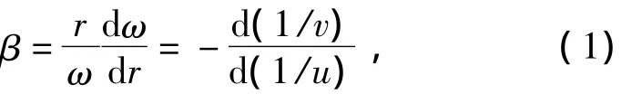
whereωis the frequency of acoustic signal,ris the range from the source,βis the waveguide invariant,whose value is 1 in the Pekeris waveguide[15],vanduare the average phase velocity and the average group velocity,respectively.
Therefore,βcan be predicted using Eq.(1)by modeling the acoustic field to get the mode phase velocity and group velocity if the information on the ocean environment is prior known accurately,which is difficult in practice.However,the first term in Eq.(1)shows that based on the image processing the value ofβcan be estimated by extracting the slope of the interference fringes in LOFARgram,which is obtained by STFT.
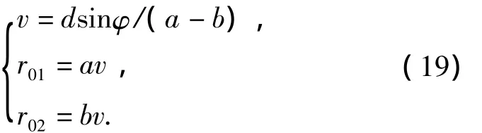
The origin of coordinates is located at the acoustic center of the single sensor or the array.Provided that the target radiates continuously broadband signals and moves in a uniform rectilinearity,the linear speed isv,the range at the closest point of approach(CPA)isr0,the corresponding time ist0,θis target bearing,andφis the heading angle which is defined as the angle between the positive axis ofxand the target moving direction.The geometry relation of target movement is shown in Fig.2.The moving trajectory of the target can be expressed as:

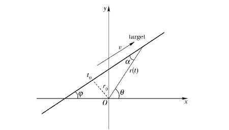
Fig.2 Moving geometry relation of target

It can be seen from Fig.2 that:
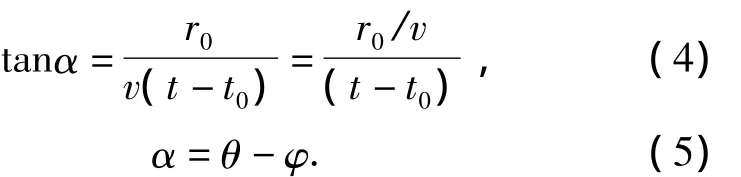
It can be derived from Eq.(4)and(5):

The slope df/dτof the interference fringes can be written as:

And Eq.(1)can be expressed as:
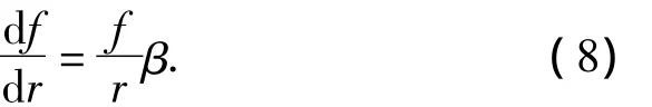
It can be known from Eq.(3)that

Substituting the Eq.(8)and Eq.(9)into Eq.(7),we have

Then both the sides of the above equation are integrated and rearranged,we have

Eq.(11)is just the trajectory equation of the interference fringes,which indicates that the interference fringes are a family of quasi-hyperbolas in shallow water.Whenβμ1,Eq.(11)can be simplified as a standard hyperbola equation in which apex is(t0,f0),wheref0is the frequency corresponding toτ=0,namely,f(0)=f0.
2 Parameter Estimation via Hough Transform
Hough transform[16]is an image processing method for edge detection,which is suitable to detect arbitrary curve.The Hough transform is to map the points on the same curve in the image space onto a family of curves intersected at a point in the parameter space,and the coordinate of the intersection reflects the parameter of the curve in the image space.The intensity of each element(a,b)in the parameter space is the cumulative intensity of the points on the curve characterized by the parameters(a,b)in the image space,so the parameters of the curve can be achieved by searching the maximum element in the parameter space.
In this paper,Hough transform is used to process the LOFARgram and bearing-time records to estimate the parameters.For the former,LOFARgram is just the image space mentioned above,in which the curves are determined by Eq.(11).Provided thatt0andf0can be gotten directly from the LOFARgram,while the parameter space is a plane which takesr0/vas the horizontal axis and the waveguide invariantβas the vertical axis.Similarly,for the latter,the bearing-time record is an image space,in which the curves are determined by Eq.(6),while the parameter space is a plane which takesr0/vas the horizontal axis and the heading angle as the vertical axis.
The simulation results of LOFARgram and its Hough transform are shown in Fig.3.The Hough transform of LOFARgram are performed fort0=0 s andf0=637 Hz as the apex of some interference fringe,as shown in Fig.3(b)and Fig.3(c).Then the parameters can be estimated by searching the maximum element in the parameter space:β=0.97 andr0/v=99.2,where the true value ofr0/vis 100,which indicates that Hough transform has high accuracy.The curve shown in Fig.3(a)as the dotted line can be achieved by substituting the estimated parameters into Eq.(11),which coincides with the bright fringe in LOFARgram.

Fig.3 LOFARgram and the results of Hough transform
Assuming that the heading angle of target is 30°,and the targets moves from far to near then the opposite,the remaining conditions are the same as the above.The bearing-time records estimated by acoustic intensity average using the vector sensor are shown in Fig.4(a).In the same way,the bearing-time records are processed by selectingt0=0 as a reference and the Eq.(6)as the Hough transform template,and the parameter space is shown in Fig.4(b).φandr0/vcan be estimated synchronously by searching the brightest pix of parameter space,they are 30°and 100 s,respectively,and the latter is exactly equal to the true value.But in practice,the bearing estimate differs from the real value by several degrees in bearing-time records,so there will be a corresponding estimated error with the parameters we concerned.

Fig.4 The Bearing-time records and the result of Hough transform
3 The Principle of Passive Ranging Using Double Array(Element)
From Eq.(11)and the parameter estimation discussed in the previous section,it can be seen that only the ratio ofr0/vcan be obtained by a single vector sensor or a single array.Therefore,the problem of passive ranging can not be solved entirely.So the model of double element or double array is adopted to realize the passive ranging,which has a far detecting range and a lot of application aspects,such as shore station,surface ship or submarine.
A double array element model is adopted as an example to explain the ranging principle,the principle using double array is the same as the former,but its operating range is father and the direction finding is more accurate.The ranging model is shown in Fig.5.The two array elements are placed onxaxis,and the array element spacing isL=d.Assuming that the target moves in a uniform linearity,its speed isv,and its heading angle isφ.The distances from the target to element 1 and 2 arer1andr2,and the corresponding bearing angles areθ1andθ2,respectively.Relative to element 1 and element 2,the ranges at the closest point of approach(CPA)arer01andr02,and the times at CPA aret01andt02,respectively.If the origin is used as a reference,the range at CPA and the time at CPA arer0andt0,respectively.

Fig.5 Double element based positioning model
LOFARgram 1 and LOFARgram 2 can be achieved by processing the signals received by element 1 and 2 using STFT.At the same time,the bearing-time records 1 and bearing-time records 2 can be achieved by bearing estimation.The four figures are the premise of further passive ranging.Four ranging algorithms will be introduced in the following sections.
3.1 Algorithm 1
The time delayTof the target moving from pointAto pointBshown in Fig.5 can be estimated by putting image cross-correlation,also called two-dimensional correlation,on two LOFARgrams,at the same time,t01andt02can be gotten easily.The heading angle can be estimated using Hough transform to process some bearing-time records,and the average value ofφ1andφ2can be adopted if Hough transform have be done to both the bearing-time records.So the navigation speed of the target can be expressed as:

Because the element spacingdis known,the speedvcan be estimated using Eq.(12).
The Hough transform of two LOFARgrams can be done to estimater01/vandr02/v:

whereaandbare the values obtained by searching a maximum in parameter space of Hough transform.The ranges at CPA relative to two elements are

Therefore,the range at CPA of target relative to the origin can be expressed as:

And the time at CPA relative to the origin is

So the horizontal distance of target is

The above equation can be used to estimate the horizontal distance of target.The advantage of this algorithm is simple,but the ranging accuracy is poor when the heading angle of target is close to 90°,and it is inapplicable forφ=90°.
3.2 Algorithm 2
Similarly,the heading angleφcan be estimated by processing the bearing-time records using Hough transform,then the ratios of the ranges at CPA relative to two elements to the target speed can be obtained by processing the LOFARgrams using Hough transform,which areaandb,respectively.The simultaneous equations are as follows:

The solution of the above equations is
Based on the Eq.(19),the horizontal range of target can be estimated by Eq.(15),(16)and(17).
This algorithm is also simple,and its calculation amount is less without image correlation.It is suitable to ranging forφ=90°,and the larger the heading angle is,the better the ranging accuracy is.However,the accuracy is poor when the heading angle is small(for example,the target is near the axial direction of the array),and the algorithm is inapplicable forφ=0°.In addition,it can be seen from the first equation of Eq.(19)that the robustness of this algorithm is poor because the target speed is determined by the difference betweenaandb,and the estimated errors caused by Hough transform are random.
3.3 Algorithm 3
The heading anglesφ1andφ2,and the ratiosmandnof the ranges at CPA relative to two elements to the target speed can be estimated synchronously by processing the bearing-time records using Hough transform,we have:

The next step of this algorithm is the same as Algorithm 2.We have

Then the following steps are also the same as the algorithms mentioned above.
3.4 Algorithm 4
This algorithm is obviously different from the algorithms mentioned above.It utilizes the definition of the waveguide invariant.
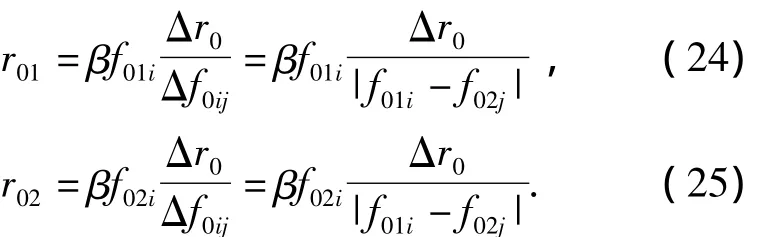
Similarly,the waveguide invariantβandr01/v=acan be estimated synchronously by processing LOFAR-grams using Hough transform,and the heading angleφandr01/v=ccan also be obtained by processing the bearing-time records using Hough transform.So the difference of ranges at CPA relative to two elements Δr0can be expressed as:

The frequenciesf01iandf02j,whereiandjare the numbers of interference fringes,of the corresponding interference fringes at CPA can be extracted easily from two LOFARgrams.So the frequency difference of the corresponding interference fringes can be expressed as:

Therefore,it can be seen from Eq.(8)that the ranges at CPA of target relative to each element are as follows:
In this way,the range at CPA relative to the origin can be estimated as:

and the navigation speedvLandvbof the target are expressed using Eq.(27)and(28),where the subscripts denote the ratio of the range at CPA to the target's speed used to estimate the speed is estimated by processing the LOFARgram or the bearing-time records.

Finally,the range of the target can be expressed as:

wherercan be estimated by=vLand=vb,respectively,and the average value of two results is used as the final estimation of target range.The range of the target can also be obtained directly by substituting=(vL+vb)/2 into Eq.(29).
4 Simulation Research
The simulation researches have been conducted to verify the correctness of four algorithms proposed above and to evaluate the ranging accuracy of each algorithm.
The conditions used in the simulation are as follows:the Pekeris model is used.The sea depth isH=55 m.The acoustic velocity and the density of water arec1=1 500 m/s andρ1=1 000 kg/cm3,respectively.While the acoustic velocity and the density of bottom medium arec2=1 610 m/s andρ2=1 900 kg/cm3,respectively.The effect of absorption is negligible.The depth of the vector sensors arezr=30 m,the element spacing isd=120 m.Supposing that the target cruises in the same depth which iszs=4 m,the speed of navigation isv=12 m/s,and the range at the CPA isr0=1 320 m.The time at the CPA is set as 0 time,and the time is defined negative when the target moves towards the receiver,and vice versa.The heading angle is 30°.The working band is 300 ~1 000 Hz.The acoustic field is modeled using the KRAKENC program.
It can be known from the above analysis that the advantage of Algorithm 1,of which ranging accuracy is dependent on the time delay estimation accuracy is to estimate the range of target at the heading angle of 0°.The time delay estimation results obtained by image cross-correlation under different heading angles are shown in Tab.1,whereτ,and Δτare the true value,estimated value and the relative estimated error of the time delay,respectively.The results indicate that,when the heading angle is 0°,the relative estimated error is 0 which causes the high ranging accuracy,and the time delay estimation accuracy roughly reduces with the increase in heading angle.If the range accuracy is required to be better than 15%,then the condition for Algorithm 1 is that the heading angle is smaller than 10°.

Tab.1 Time delay estimation results obtained by image cross-correlation under different heading angles
Ranging results and relative errors of four algorithms when heading angles are 10°,30°and 90°are shown in Fig.6 to Fig.8,where(a)of each figure shows the ranging results,while(b)shows the corresponding relative ranging errors.It can be seen from the comparison of the results in the figures that:first,the relative ranging error of Algorithm 1 is about 9.2%when the heading angle is 10°,while the error is about 23.4%when the heading angle is 30°,which once again verifies that Algorithm 1 is suitable for small heading angle,especially for 0°heading angle at which Algorithm 2,3 and 4 are inapplicable.Second,Algorithm 2,3 and 4 have enough passive range accuracy when the heading angle is large,and the general trend is that the larger the heading angle is,the better the range accuracy is.

Fig.6 Ranging results and relative errors of four algorithms at 10°heading angle
5 Conclusions
The stable interference structure of the low-frequency continuous spectrum acoustic field has been observed in the sea trials.For a target moving towards a receiver from far to near,and then moving away form the receiver,the equation of the interfe-rence fringes has been derived based on the concept of waveguide invariant and the geometric relationship of target moving trajectory,indicating that the interference fringes are a family of quasi hyperbolas.The heading angleφ,waveguide invariantβandr0/v(wherer0is the target's range at CPA andvis the target speed)can be estimated by processing the LOFARgram and the bearingtime records using the Hough transform.The double element or double array model is adopted to achieve passive ranging,four ranging algorithms are proposed.The simulation research shows that Algorithm 1 is suitable for the scenario of small heading angle,the ranging error is less than 10% if the heading angle is smaller than 10°.Algorithm 2,3 and 4 are inapplica-ble when the heading angle is equal to 0°,but all of them have enough range accuracy when the heading angle is larger than 10°.In the practical application,the heading angle should be estimated first,and then a threshold is set according to heading angle in order to use a suitable ranging algorithm.

Fig.7 Ranging results and relative errors of four algorithms at 30°heading angle
A complete interference fringe is required to range for all the four algorithms which do not fully satisfies the operational requirements of sonar device,but they are still valuable for basic research and have important application prospect in many aspects,such as shore station,airborne sonobuoy,marine research,especially acoustic measurement and so on.More detailed simulation and sea trial research will be needed for their practical engineering applications.The ranging algorithm suitable for the scenario without the closest point of approach is the focal point of further research.
[1]WANG Xin-yong,HUI Jun-ying,YU Hong-xia.Filtering applied research on noise passive ranging[J].Journal of Harbin Engineering University,2005,26(1):80 - 83.(in Chinese)
[2]WANG Yan,HUI Jun-ying,LIANG Guo-long.Target motion analysis based on bearing and time delay difference of dual arrays[C]∥Proceedings of National Conference on Underwater Acoustics,Shanghai:Editorial Office of Technical Acoustic,2001:60-62.(in Chinese)
[3]Thode A M,Kuperman W A,D’Spain G L,et al.Localization using Bartlett matched-field processor sidelobes[J].J Acoust Soc Am,2000,107(1):278-286.
[4]HUI Juan,HU Dan,HUI Jun-ying,et al.Research on the measurement of distribution image of radiated noise using focused beamforming[J].Acta Acoust,2007,34(2):356-361.(in Chinese)
[5]YU Yun,MEI Ji-dan,ZHAI Chun-ping,et al.Sea trial researches on the measurements of passive source space distribution imaging and positioning[J].Acta Acoust,2009,32(4):103-109.(in Chinese)
[6]HUI Jun-ying,SUN Guo-cang,ZHAO An-bang.Normal modes acoustic intensity flux in Pekeris waveguide and its cross spectra signal processing[J].Acta Acoust,2008,33(4):300-304.(in Chinese)
[7]YU Yun,HUI Jun-ying,Zhao An-bang,et al.Complex acoustic intensity of normal modes in pekeris waveguide and its application[J].Acta Physica Sinica,2008,57(9):5742-5748.(in Chinese)
[8]Chuprov S D.Interference structure of acoustic fieldin the layered ocean[M]∥Brekhovskikh L M,Andreeva I B,Ocean Acoustics Nauka,Moscow:Modern State,1982:71-91.
[9]D’Spain G L,Kuperman W A.Application of waveguide invariants to analysis of spectrograms from shallow water environments that vary in range and azimuth[J].J Acoust Soc Am,1999,106(5):2454-2468.
[10]Rouseff D,Spindel R C.Modeling the waveguide invariant as a distribution[J].AIP Conference Proceedings,2002,621(1):137-160.
[11]Goldhahn R,Hickman G,Krolikc J.Waveguide invariant broadband target detection and reverberation estimation[J].J Acoust Soc Am,2008,124(5):2841 -2851.
[12]Quijano J E,Zurk L M.Rouseff D.Demonstration of the invariance principle for active sonar[J].J Acoust Soc Am,2008,123(3):1329-1337.
[13]Turgut A,Orr M,Rouseff D.Broadband source localization using horizontal-beam acoustic intensity striations[J].J Acoust Soc Am,2010,127(1):73-83.
[14]Cockrell K L,Schmidt H.Robust passive range estimation using the waveguide invariant[J].J Acoust Soc Am,2010,127(5):2780-2789.
[15]Brekhovskikh L M,Lysanov Y P.Fundamental of ocean acoustic[M].3rd ed.Moscow,Russia:AIP Press,2002:143-146.
[16]Hough P VC.A method and means for recognizing complex patterns:US,3069654[P].1962-12-18.
[17]HUI Jun-ying,HUI Juan.Fundamental theory of signal processing in acoustic vector field[M].Beijing:National Defense Industry Press,2009:10.(in Chinese)

- Defence Technology的其它文章
- Study on Effects of Diesel Engine Cooling System Parameters on Water Temperature
- A New Fusion Method for Conflicting Evidence
- Numerical Simulation and Performance Analysis on Windmill Starting Process of Small Turbojet Engine
- New Wideband Beam-forming Method Used in Underwater Communication System
- Research on Estimation of Time Delay Difference in Passive Locating for Impulse Signal
- Reliability Sensitivity Analysis for Location Scale Family