
Statistical Model for Intensities in the Rotational Spectra of Linear and Non-Linear Molecules
2011-12-12 02:43SAIZAndr
物理化学学报 2011年5期
SAIZ Andrés
(Departamento de Matemática Aplicada,Universidad Politécnica de Valencia,Escuela ETSGE,Camino de Vera s/n, Valencia 46022,Spain)
1 Introduction
Spectral lines of molecules in infrared and microwaves are produced by rotation and vibration,and they represent the lowest quantized energy modes of molecular motion.The analysis of the rotational spectrum is an accurate way to determine the structure of a molecule in the gas phase.Non-linear molecules can be recognized by their related values of the three principal moments of inertia,IA,IB,IC.In the asymmetric top molecule cases,the three principal moments of inertia are unequal.Because of that,the rotational motion produces a very complex rotational spectrum.A good introduction to molecular spectroscopy can be found in several books.1-3
Some different ways are explored when a statistical description of the spectrum is desired:
(1)The study of the distribution of the spacing between eigenvalues of the energy operator.These spacings are often extracted from experimental data and the statistical measurements commonly used are spectral distribution(probability of finding an energy level in the vicinity of an interval related to an existing energy level)and level spacing probability distribution(probability of finding two consecutive energy levels at a certain distance).Fluctuation properties of complex spectra are described according to Wigner′s random matrix theory(RMT). These fluctuations appear in spectra of many physical systems and seem to be highly universal.
(2)The study of the spectral phenomenon from the dimensional point of view.The studied measurements have been the intensity4and the distribution of the measure in the wavelength domain5.
(3)The study of intensities in transitions of molecules6-10or intensities as molecular descriptors11.
In this paper we look for similarities among different spectra.With this aim,we propose the study of spectral lines according to the density of probability of finding intensities in a range of intensities,as it was previously studied in literature.12
2 Analyzed spectra from non-linear molecules
The spectral lines of organic and inorganic molecules have been obtained from the Jet Propulsion Laboratory(JPL)Molecular Spectroscopy Team.13These lines are mainly rotational lines,but it is not warranted that these spectra are purely rotational.Also,incompleteness of spectra should be taken in consideration,because intensities of vibrational states in general are not in the JPL catalogue.
The non-linear molecules studied are the following:acrylonitrile(C2H3CN),75697 lines;dimethyl ether(CH3OCH3),21735 lines;hydrogen peroxide(H2O2),38357 lines;peroxynitric acid (HOONO2),50775 lines;butyronitrile(C3H7CN),131349 lines; nitrogen dioxide (NO2), 16444 lines; ethyl formate (C2H5OOCH),60671 lines;nitric acid(HNO3),36551 lines; ethyl cyanide(C2H5CN),52883 lines;nitrosylhydride(HNO), 10293 lines.For each line we have the frequency in MHz,and the integrated intensity in nm2·MHz at 300 K from theoretical arguments based on Boltzmann and Bose-Einstein statistics. The range of frequencies of the lines of each molecule is different in each case,but all of them between 102and 10-1MHz.
In this section we analyze the behavior of P(I),the probability density function(PDF)of finding one intensity.With this aim we are going to utilize histograms,which are the classic tool to estimate P(I)from experimental data.They provide a consistent estimate of the true underlying PDF,but this is only achieved when the choice of the number of bins is adequate.It has been shown in literature14that an optimal bin size histogram,which provides an unbiased estimation of the PDF,is reached when

where W is the width of each bin,σ is the standard deviation and N is the number of available samples.For practical purposes we use the estimated standard deviation.
Each set of intensity data from a molecule has a maximum intensity,I,and a minimum intensity,I,where j is the number of molecules,j=1,2,…,10.Thus,the optimal number of bins for each molecule is:
where Int stands for the integer part.This allows us to create the set BNLgiving by:
Hence,the probability that an intensity lies in a bin i(i=1, 2,...,bj)from a molecule j(j=1,2,…,10)is pij(I)=nij(I)/Nj, where nij(I)is the number of intensities lying in a bin i from a specific molecule j,and Njis the total number of intensities in the spectrum of this molecule.
We choose<I>,the average of intensities in each bin,as a close representative of the internal distribution of intensities in each bin.If other election is made,graphical representation is not correct due to the log-log representation.In Fig.1 we represent P(<I>)vs<I>for all molecules.As we can see in Fig.1, P(<I>)curves are very similar.They could be fitted by power laws with exponential tails such as P(I)=αI-βexp(-γI).
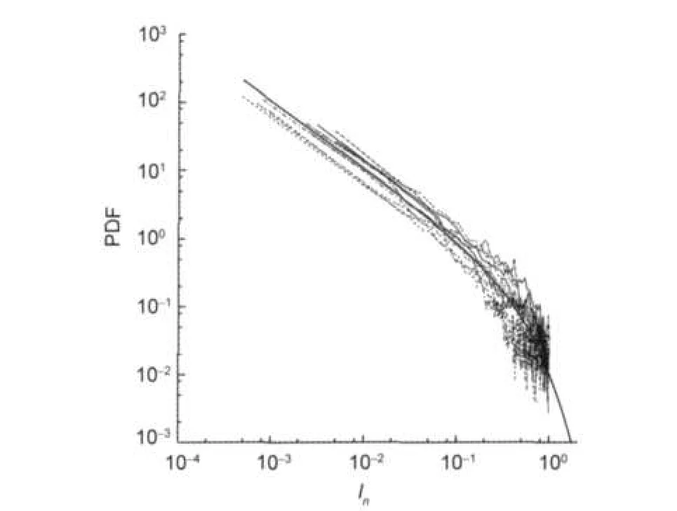
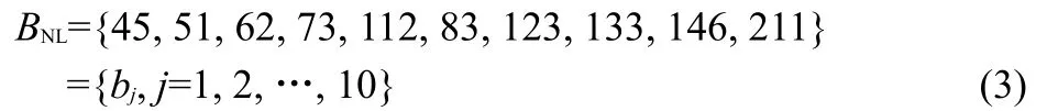
Fig.2 Log-log plots of the linear interpolated data for the intensity(PDF vs In)This picture shows all 10 molecular spectra studied.The curve ρ(In)=0.11In-0.99exp(-2.4In)(thick line)is a nonlinear least-squares approximation to the data.
Since data from molecules lead to similar curves,we propose two convenient variables,Inand Ic,in order to group them around a general curve that will be given in Section 4.The aim of this is to study relations between them.Specifically,we look for a process able to explain the dispersion of such curves respect to the general one.
Firstly,as an approximation,we define the variablewhere its PDFs are denoted byIn Fig.2 we see how this variable groups the curves.
Secondly,we define another convenient variable,Ic=<I>/W, where its PDFs are denoted bydoes not depend on any specific scale.Notice that its integer part plus one is the number of the bin to which Icbelongs.In Fig.3 we represent the curves for the new variable Ic.
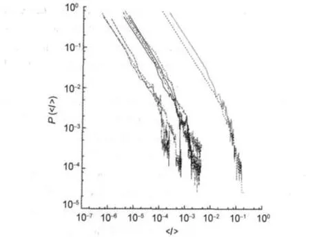
Fig.1 Log-log plots of the linear interpolated data for the mean intensity P()vsThis picture shows all 10 molecular spectra studied.
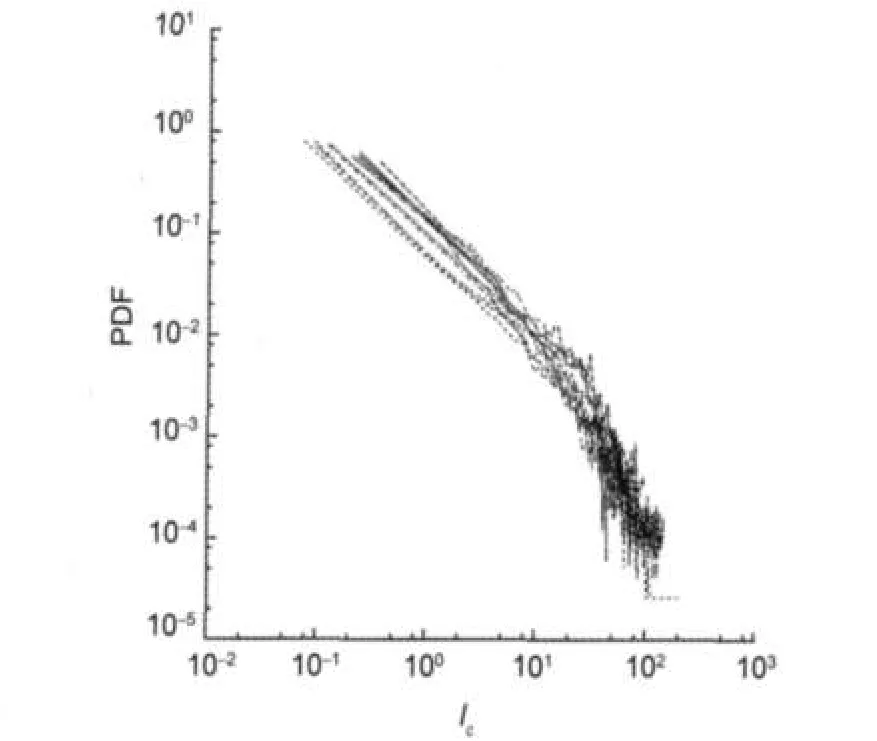
Fig.3 Log-log plots of the linear interpolated data of the studied molecules(PDF vs Ic)This picture is Fig.1 transformed after using Ic.
In order to analyze the existence of a process able to explain the dispersion of the curves in Fig.3,we estimate the standard deviation,σI,and the average,µi,of the different PDFs′,in the same bin i,for all possible j(less than or equal to 10). The points,(µ,σ(µ)),that representµiand σifor all bin i,can be fitted by σ=0.55µ,see Fig.4,that is a behavior consistent with a lognormal distribution,as we will see in the following.
There are 10 or less samples per bin.Thus,in order to have more samples we will rebuild the statistical process considering that all the bins are equally distributed,but with σ depending onµ.In this case,we can construct a kind of typified variablewhere 1≤j≤10,and i=1,2,…,bj,is the number of bin.We can compare distributions using this variable.In each bin i the mean and the standard deviation behave as<M>i= 1 and σ(M)i≅0.55 respectively,except for the less populated bins.In these conditions,assuming the same distribution inside bins,we can group all data.In this way,we create a sort of bin in which all the samples join together.Hence,we can rename the variable Mijjust as M,where M∈[0.0895,3.3].
We create a histogram in M following the equation(1).The width of each bin is 0.16,hence,the number of bins is 20.We show the PDF of the process in the Fig.5.This PDF is consistent with a lognormal process,as:
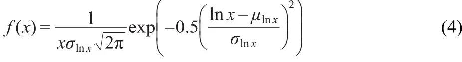
where the parameters of the lognormal distribution σlnxand μlnxare:
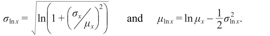
In our case σ(M)=σx=0.55 and<M>=µx=1,so σlnx=0.5141 and µlnx=-0.1321.
As shown in Fig.5,the variable M has a distribution consistent with a lognormal process.This behavior is directly suggested by σxandµx.
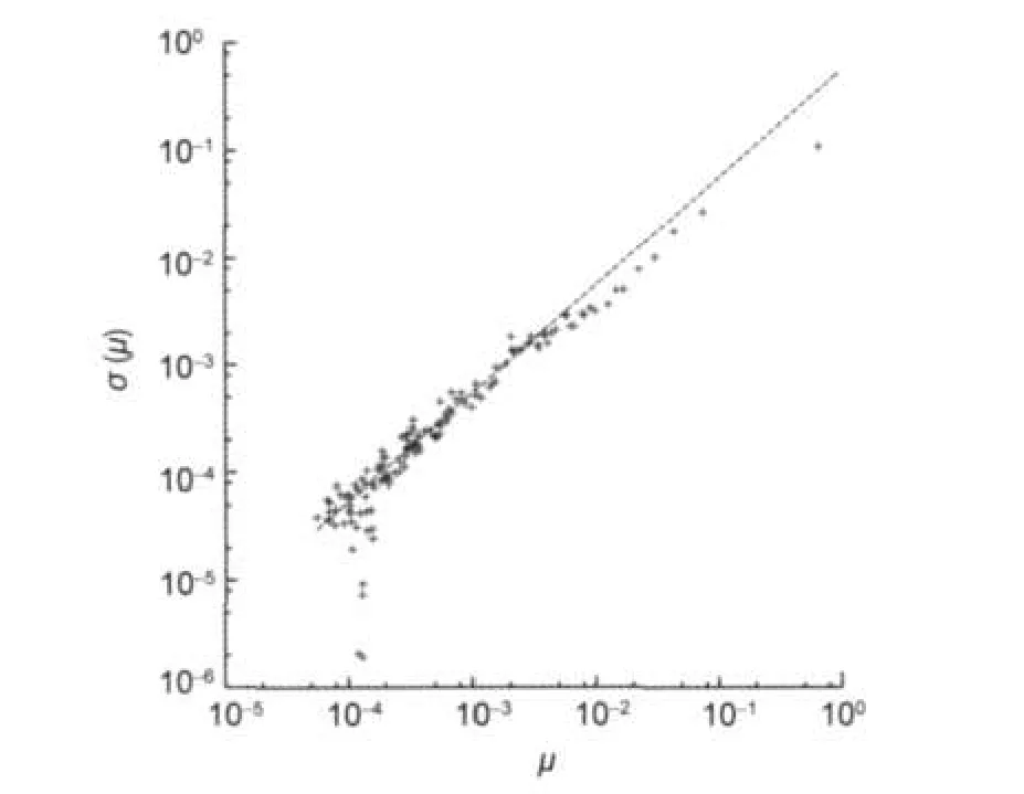
Fig.4 Typical deviation σ vs average of PDF in each bin(µ)of the same process for all 10 moleculesDotted line is σ=0.55µ.
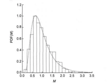
Fig.5 Histogram of the variable PDF(M)vs M and lognormal curve when
The variable M helps us to superpose distributions which,if significantly different in each bin,do not show a lognormal distribution.Therefore,it seems reasonable to consider a common process as the origin of the dispersion in curves ρc(Ic).As an approach to the general curve,we can create an‘average curve’with the average values of ρcand Icin each bin.This shows a good agreement with a power law with exponential tail,as ρc(Ic)=aIc-bexp(-cIc)where a=0.11,b=0.99,and c=0.02,see Fig.6.
Since the curves seem related we proceed to study the dispersion and the mean.The variables Icand Inhelp us to identify the origin of the dispersion.Its densities are related according to:
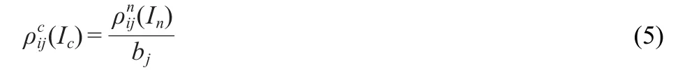
where j=1,2,…,10,represents the molecules and i=1,2,…,bjthe number of bin.Therefore,the standard deviation and the averages are expressed by:
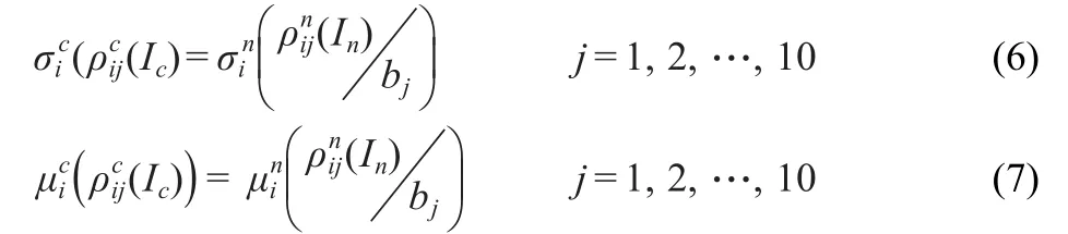
Fig.6 Log-log plot for the average data Icand ρc(Ic)in each bin(crosses)Fitted curve is ρc(Ic)=0.11Ic-0.99exp(0.02Ic).
Let us consider that the behavior ofis,where k stands for the constant behavior for all the molecules and v stands for the variable behavior.Let us consider too thatis smaller thanand it can be ignored compared with it.In that case we have:andIn this way we have a first approximation to the contribution of this factor to the dispersion.Therefore,
it is close to the experimental fit,whereandare computed from the inverse of the elements of the set BNL(3).In the considered case,the most important part of the dispersion comes from the different number of bins considered in each spectrum.
The above results are coherent with the idea that a general law may exist and the curves ρc(Ic)and ρn(In)derive from it following the suggested dispersive process.
3 Analyzed spectra from linear molecules
Spectral lines from linear molecules have been obtained from the JPL Molecular Spectroscopy Team,13as in Section 2. They are the following:Br-79-O,1892 lines;PS,2340 lines; AlCl,11525 lines;ClO,2585,NS,2402,PNv=0-4,1637 lines; NO,1909 lines;O-17-O,10787 lines;SiC-13,2417 lines; NS-34,2362 lines;Cl-37-O,2624 lines;AlCl-37,11326 lines.
Using same procedures as in Section 2.1,the optimal number of bins for each molecule allows us to generate the set BL:

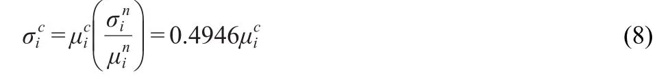
When we make representations of spectra of linear molecules we find different behaviors.In Fig.7 we can observe different shapes of these spectra.They are grouped,after adequate shifting of P(I),in order to achieve collapse of curves.In that case the fit to a common behavior can not be made.
In some cases similarities could be attributed to isotopes,but Fig.7(b,d)shows non isotopic molecules also.
4 Boltzmann distribution
So far we have used power laws with exponential tails in order to approximate a curve to the behavior of the PDF of the intensity of spectra.These kinds of curves,with an explicit expression,are convenient in order to approach the functional behavior of curves.Nevertheless,power laws with exponential tails have basic problems.For that kind of curves a maximum in intensity is not allowed.This seems to be a serious limitation for a realistic description of a physical phenomenon as the spectrum is.Other disadvantage is scaling.These kinds of curves do not show scaling in the variable intensity.
In Fig.7 we observe different behaviors for linear molecules. These intensities of spectra,after adequate shifting,collapse into common behaviors.This fact suggest a spectrum model in which each molecule should be associated to a parameter which corresponds to a spectrum.
A first approach to the shape of P(I)is a model based on the Boltzmann distribution.15This distribution is the classical distribution function for an amount of energy which distributes among identical but distinguishable particles,and arises in statistical mechanics,specifically in equilibrium systems(see literature16for a revision of this item).Atomic,ionic or molecular levels obey that distribution.
Fig.7 Log-log plots of P(I)vs I of spectra of linear molecules(a)molecules O-17-O,NO,and SiC-13;(b)molecules Br-79-O,AlCl,PNv=0-4andAlCl-37;(c)molecules NS and NS-34;(d)molecules PS,ClO,and Cl-37-O
The Boltzmann distribution for continuous systems is described by f(E)=exp(-βE),where β=1/kBT,kBis the Boltzmann′s constant,T is the temperature(T=300 K in this paper),and E is the energy level.Thus,ρ(E)=Ng(E)f(E),where N is a positive constant and g(E)≥0 is the multiplicity of level E,describes the density of states of the system.
In order to give a description of spectra of linear and non-linear molecules,let us consider the following approach to the problem.
4.1 Relevance of multiplicity g(E):statistical arguments
If we assume that in molecules at room temperature all degrees of freedom are decoupled then,summing over all molecular states is equivalent to summing over all possible translational,rotational,vibrational and electronic states.Thus,the molecular partition function,qmol,assuming continuum,is:

where g(E)is the multiplicity and qtrans,qrot,qvib,and qelecare partition functions related to translational,rotational,vibrational, and electronic states,respectively.
Partition function is temperature dependent.It is in such a way that at low temperature not all degrees of freedom contribute significatively to its corresponding partition function.For example,at room temperature,qtrans~1026-1028,qrot~19,qvib~1, and qelec~1.
Also,partition function is useful in the study of thermodynamic functions,as molecular energy Emol=NkBT2(∂ln(qmol)/∂T)N,V. At room temperature qtransand qrotare the most contributing partition functions to qmol,but qtransdoes not take part in spectra generation.They scale with temperature as:qtrans∝T1/2and qrot∝T1/2for each degree of freedom.Thus,in this paper we suppose that qmolscales as qmol∝Tw/2,where w is the number of active degrees of freedom,and includes participation of rotational levels to spectra,but without translational contributions.Multiplicity in equation(10)must be coherent with this fact.
In order to reproduce the scaling behavior of qmol,we propose the following multiplicity:

where Im(maximun intensity),b>0 and s>1.In that case,equation(10)becomes:
where Γ is the standard gamma function.If we indentify w=s+ 2 we can observe that the dominant part of qmolscales as Tw/2when Imis sufficiently small.The election of equation(11)is the simplest election we can reproduce the expected behavior for qmol.The term Imis needed in order to have a maximum intensity.In Section 5 we will study the behavior of more elaborated g(E)that finally leads to a similar behavior.
4.2 Building a P(I)
In the present case we assume that intensities I(E)are approximately proportional to ρ(E).This is a good approximation because transitions have specific rules with constant probabilities.Thus:

whereA is a constant.We will considerA=1 for computing.
Let us consider dp(I),as the probability of finding an intensity in[I,I+dI].In a general way dp(I)is:

where m represents the number of intervals that contribute to dp.
P(I),the PDF associated to dp(I)is:
where g′(E)/g(E)-β≠0 and g(E)≥0 for all E.
A parametric representation of P(I),(I,P(I)),with parameter E,may be easily found in some cases.15
As a first approach to the shape of spectra of non-linear molecules one can consider g(E)=Enwith n=-1.15In that case the shape of these spectra is correctly reproduced,see Fig.8.Nevertheless,a multiplicity as g(E)=Encannot reproduce shapes of spectra of linear molecules.Also,in experimental spectra,a cutoff in intensities due to the non existence of arbitrarily large intensities is observed.Intensities above certain Imare not detected.
In the next section,in order to give an explanation to shapes of spectra of linear and non-linear molecules,we will use the multiplicity introduced in equation(11).
5 Theory and experiment data
In order to have a more compact and clear description of properties derived from multiplicity of equation(11)we consider the following change of notation on that multiplicity:

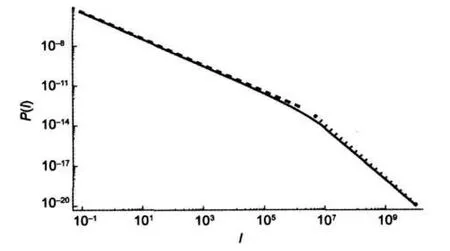
Fig.8 Log-log plot of P(I)vs I thin line:g(E)=En,n=-1,and β=3×10⁶;dashed line:P(I)=3.5×10⁻⁷I-1; dotted line:P(I)=1.1I-2
where ξ=b/Im,Im>0,E≥0,ands∈Z+.I=Imwill be the maximum observed intensity when I(E)is a decreasing function.In that case I′(E)<0,that is,g′(E)-βg(E)<0.Notice that g′(E)-βg(E)≠0 in this paper.Near to Ei,such as I′(Ei)=0,P(I)grows significatively.Experimentally,this grows will be limited because E is quantized.Another feature related to equation(16)is the behavior when I→0.In that case,P(I)behaves as I-1.15
Let us study the functional form of P(I)generated from the multiplicity of equation(16)when β=0.3,Im=90 and s=5 are used.Different curves with various ξ have been computed, some of those curves appear in Fig.9.
ξc=2.415/90,is the numerically computed critical value of ξ, such as when ξ=ξc,a double real root of I′(E)=0 appear.When ξ≥ξc,two real roots appear,then,local Imaxand Iminfor I(E)exists,and P(I)diverges at these points.In those cases we compute random values of E using an inverse transform sampling, and compute P(I)from simulated values of I.In Fig.10(a)we show P(I)when ξ is close to the critical value,ξc.In Fig.10(b) we show a simulation of 106samples of E when ξ=10/90.Thus, the same number of samples of I is obtained,and then,the shape of P(I)is generated.Notice that the two peaks of P(I)on Fig.10(b)correspond to the two local extremes of I(E).
The power s in equation(16)is also an important parameter. In Fig.11 we represent two different P(I)curves for values s=5 and s=6.Notice how tiles of such a curves increase with s.
For a specific s a family of P(I)depending on parameter ξ have been obtained.Now,we need to fit obtained curves to experimental spectra of linear and non-linear molecules.Let us consider β=0.3,s=5 and Im=90,for other values of s curves of similar shape were obtained.With these values we compute some curves with various ξ.After this,we shift curves adequately in order to reach coincidences in log-log plots.Obtained results are shown in Fig.12.One can see a good agreement among experimental and theoretical curves in spectra from linear and non-linear molecules.In Fig.12(c),linear molecules of Fig.7(d)has been represented vs its theoretical prediction.Species from down left panel of Fig.7 could be easily reproduced in the same way changing ξ.
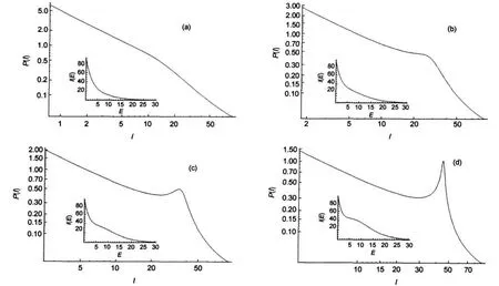
Fig.9 Log-log plots of P(I)vs I depending on ξIn insets we show I(E)=g(E)exp(-βE)where g(E)=Im(1+ξE5/2).In all the cases Im=90 and β=0.3.(a)ξ=0.4/90;(b)ξ=1/90;(c)ξ=1.4/90;(d)ξ=2/90
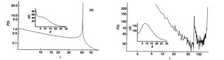
Fig.10 Log-log plots of P(I)vs I when g(E)=Im(1+ξE5/2)(a)ξ=2.41/90,near ξc,Inset:I(E)=g(E)exp(-βE);(b)simulation of 106values of I,where ξ=10/90,far from ξc;In both cases β=0.3 and Im=90.

Fig.11 Log-log plots of P(I)vs I when g(E)=Im(1+ξEs/2)thin line:s=5 and ξ=1/90;thick line:s=6 and ξ=0.22/90; In both cases Im=90 and β=0.3.
So far we used s=5,w=7 active degrees of freedom,as an adequate value in order to reproduce shapes of spectra,and in order to reproduce the dominant contributions to spectra in qmol. Nevertheless,in order to have a more rich behavior in P(I),we can suppose the existence of more non dominant terms in g(E):

where s>1 and s∈Z+.
Let us consider s=4,w=6,and the following multiplicity:

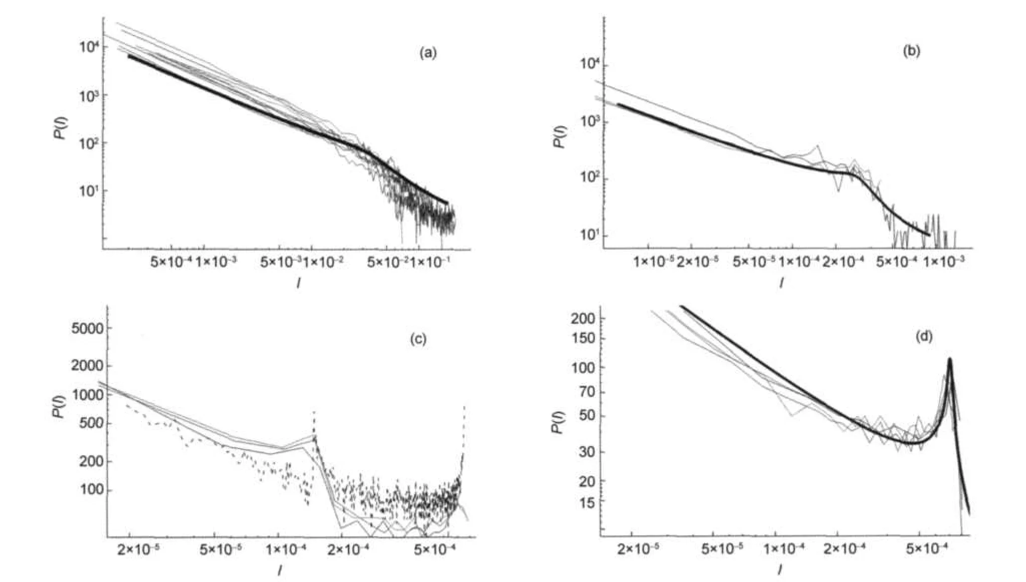
Fig.12 Theoretical behavior of P(I)vs experimental behavior(a)non-linear molecules,adjusted with ξ=0.5/90;(b)linear molecules of Fig.7(a),adjusted with ξ=1/90;(c)linear molecules of Fig.7(d),adjusted with ξ=25/90; (d)linear molecules of Fig.7(b),adjusted with ξ=2/90.In all the cases β=0.3 and g(E)=90(1+ξE5/2).Thick lines and dashed line represent theoretical behavior. It has been adequately shifted in order to reach coincidences over log-log plots.Different colors represent different molecules.
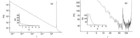
Fig.13 Log-log plots of P(I)vs I when g(E)includes the existence of more terms in E(a)g(E)=Im(1+2E2-2E);(b)g(E)=Im(1+15E2-2E);in both cases Im=90 and β=2.Also,in both cases insets are:I(E)=g(E)exp(-βE).
In that case roots E1and E2of I′(E)=0 could be computed alge-braically.If we seek for a double root E1=E2discriminant,Δ,of I′(E)=0 must be zero.

Thus,
In Fig.13 ξ3=-2 and β=2 have been used,and two possible elections of g(E)are represented.In Fig.13(a)ξ1=2,Δ=0,in order to have a double real root.In Fig.13(b)ξ1=15 has been used,Δ>0,in order to show the shape of spectra when two different real roots appear.Those cases show a similar behavior as for s=5, in Fig.10.
6 Conclusions
Analyzed spectra come from a semi synthetic catalogue in which completeness are not warranted and intensities are computed using theoretical models.Nevertheless,this catalogue is a good tool in order to test statistical models of spectra of linear and non-linear molecules.
One of the keys to the problem of finding P(I)is the multiplicity g(E).We obtain full PDF spectra when using the adequate multiplicity.In that case g(E)=Im(1+ξEs/2),is the simplest multiplicity derived from statistical arguments related to the partition function qmol.
The distribution of intensities in spectra depends on two parameters that arise in previous multiplicity:Imand ξ.Imgives the maximum intensity when I(E)is a decreasing function.ξ is the responsible of divergence peaks in P(I).When ξ<ξcno real roots for I′(E)=0 exist,when ξ=ξca double real root exist and, when ξ>ξctwo different real roots appear,and then,two divergence peaks appear in P(I).When real roots appear,theoretical prediction is slightly worse around divergence peaks.This seems to be related to the approximation to continuum considered in this paper.
Behavior of spectra of molecules has been grouped in order to give a common graphical description,but it is not guaranteed that spectra from linear or non-linear molecules behave always as shown in this paper.Shape of spectra in intensities only depends on specifics values of parameters Im,β and ξ.
An important consequence is the fact that all systems ruled by a Boltzmann distribution,satisfying similar conditions to that one described in this paper,will have a similar behavior.
Acknowledgment:To the memory of Lorenzo Ferrer.
(1) Gordy,W.;Cook,R.L.Microwave Molecular Spectra;Wiley: New York,1984.
(2) Kroto,H.W.Molecular Rotation Spectra;Dover:New Yrok, 1992.
(3) Bernath,P.F.Spectra of Atoms and Molecules;Oxford UP:New York,1995.
(4) Shalev,E.;Klafter,J.;Plusquellic,D.F.;Pratt,D.W.Physica A 1992,191,186.
(5) Saiz,A.;Martínez,V.J.Phys.Rev.E 1996,54,2431.
(6) Schlapp,R.Phys.Rev.1932,39,806.
(7) Watson,J.K.G.Can.J.Phys.1968,46,1637.
(8)Morioka,Y.;Hara,S.;Nakamura,M.Phys.Rev.A 1980,22, 177.
(9) Zemtsov,Y.K.;Starostin,A.N.JETP 1993,76,186.
(10) Finsterhölzl,H.;Hochenbleicher,J.G.;Strey,G.J.Raman Spect.2007,6,13.
(11) Bielinska,D.;Waz,P.;Basak,S.Eur.Phys.J.B.2006,50,333.
(12) Saiz,A.Revista Internacional de Sistemas 2003,13,64.
(13) Pickett,H.M.;Poynter,R.L.;Cohen,E.A.;Delitsky,M.L.; Pearson,J.C.;Muller,H.S.P.J.Quant.Spectrosc.Rad. Transfer.1998,60,883.
(14) Scott,D.W.Biometrika 1979,66,605.
(15) Saiz,A.Physica A 2010,389,225.
(16) Sears,F.W.;Salinger,G.L.Thermodynamics,Kinetic Theory, and Statistical Thermodynamics;Addison-Wesley Pub.Co.: Massachusetts,1975.
