
Effect of aggregation intervalon vehicular traffic flow heteroscedasticity
2013-12-29 02:05ShiGuogangXiangQiaojunGuoJianhuaZhangHongxin
Shi Guogang Xiang Qiaojun Guo Jianhua Zhang Hongxin
(1 School of Transportation, Southeast University, Nanjing 210096, China)(2Intelligent Transportation System Research Center, Southeast University, Nanjing 210096, China)
With the rapid economic and social development, the number of vehicles is increasing dramatically in China, causing serious congestion and safety issues for the transportation systems, in particular, for big cities. For alleviating the negative impacts associated with traffic congestion and safety issues, the conventional approach of building more roads is limited due to land use constraints. The applications of advanced technologies, such as computer technology, communication technology, database technology, statistical data mining technology, etc., into the conventional transportation systems have been receiving increasing attention from both research and industry sectors, stimulating the rapid development of the intelligent transportation systems (ITS).
Many applications have been developed under the broad umbrella of ITS and reliability-related applications can provide more robust solutions for battling the congestion and safety issues, where the uncertainty information concerning transportation systems is modeled and utilized to impart the reliable treatment into traffic management and control. In this direction, two major approaches are used to model the second-order moment of transportation information, i.e., the generalized autoregressive conditional heteroscedasticity (GARCH) model[1-4]and the stochastic volatility model[5]. In addition, Guo et al.[6]established the heteroscedastic nature of traffic information, providing a foundation for performing the abovementioned uncertainty modeling analysis.
Note that all these studies are conducted for a single time interval; however, as shown in Refs.[7-9], the aggregation interval is an essential component for transportation system applications. Therefore, in this paper, we investigate the effect of aggregation intervals on the traffic condition heteroscedasticity.
1 Theoretical Background
1.1 Aggregation interval
The aggregation interval is a critical factor for characterizing or defining traffic condition data. For example, inHighwayCapacityManual2000, a 15 min aggregation interval is usually used to compute the volume of traffic, i.e., the number of vehicles passing a road section within a single 15 min aggregation interval[10]. Similarly, other traffic characteristics such as occupancy, speed, etc. can also be defined over a certain aggregation interval. Intuitively, aggregation intervals will affect the characteristics of traffic variables series. As shown in Ref.[8], longer aggregation intervals will help to cancel out the noise and hence create a smoother traffic flow series. The effects of aggregation intervals have been investigated in other fields such as short term traffic flow forecasting and single loop speed estimation. In this paper, the effect of aggregation intervals on the traffic flow heteroscedasticity is investigated.
1.2 ARIMA modeling
For a selected aggregation interval, the collection of traffic flow data formulates a traffic flow time series, and for this data, the conventional autoregressive integrated moving average (ARIMA) model has been proven to be an effective modeling tool[11]. Given a traffic flow time series process denoted by {Xt}, the ARIMA(p,d,q) model is defined as
φ(B)(1-B)dXt=θ(B)εt
wheretis the time index;pis the order of the short-term autoregressive polynomial;qis the order of the short-term moving average (MA) polynomial;dis the order of short-term differencing;Bis the backshift operator such thatBXt=Xt-1;εtis the random error at timet;φ(B) is the short-term AR polynomial defined asφ(B)=1-φ1B-φ2B2-…-φpBp;θ(B) is the short-term MA polynomial defined asθ(B)=1-θ1B-θ2B2-…-θqBq.
In the above definition, the roots ofφ(B) andθ(B) are assumed to be outside of the unit circle and have no common factors.εtis the residual series, and for traffic flow series, it has been proven to be heteroscedastic; i.e., it has zero mean and time-varying conditional variance[6].
The ARIMA model can be processed using the conventional Box-Cox framework, which includes three major steps, i.e., model identification, model estimation, and model diagnostic check[11]. In the model identification step, the orders of the model will be selected based on the minimum information criterion. In the model estimation step, the model parameters will be estimated using primarily the maximum likelihood estimation approach. In the model diagnostic check step, the estimated model will be tested to make sure that the residuals after applying the estimated model on the data containing no autocorrelation structure. It is worthwhile to mention that the above three steps can be conducted iteratively so that the final model will meet the requirements. Since these three steps are generally complex for carrying out manually, commercial software packages have been developed to facilitate ARIMA modeling, e.g., SAS PROC ARIMA[12].
1.3 Traffic heteroscedasticity
In conventional statistical analysis models such as analysis of variance, regression, etc., the data are generally assumed to be having constant variance, or the data are called homoscedastic. However, in some cases, e.g., for the traffic flow series, the process variance is time-variant; i.e., traffic flow series is called heteroscedastic. Using traffic flow series collected in the United Kingdom and aggregated at a 15 min aggregation interval, the heteroscedastic phenomenon can be demonstrated in Fig.1.
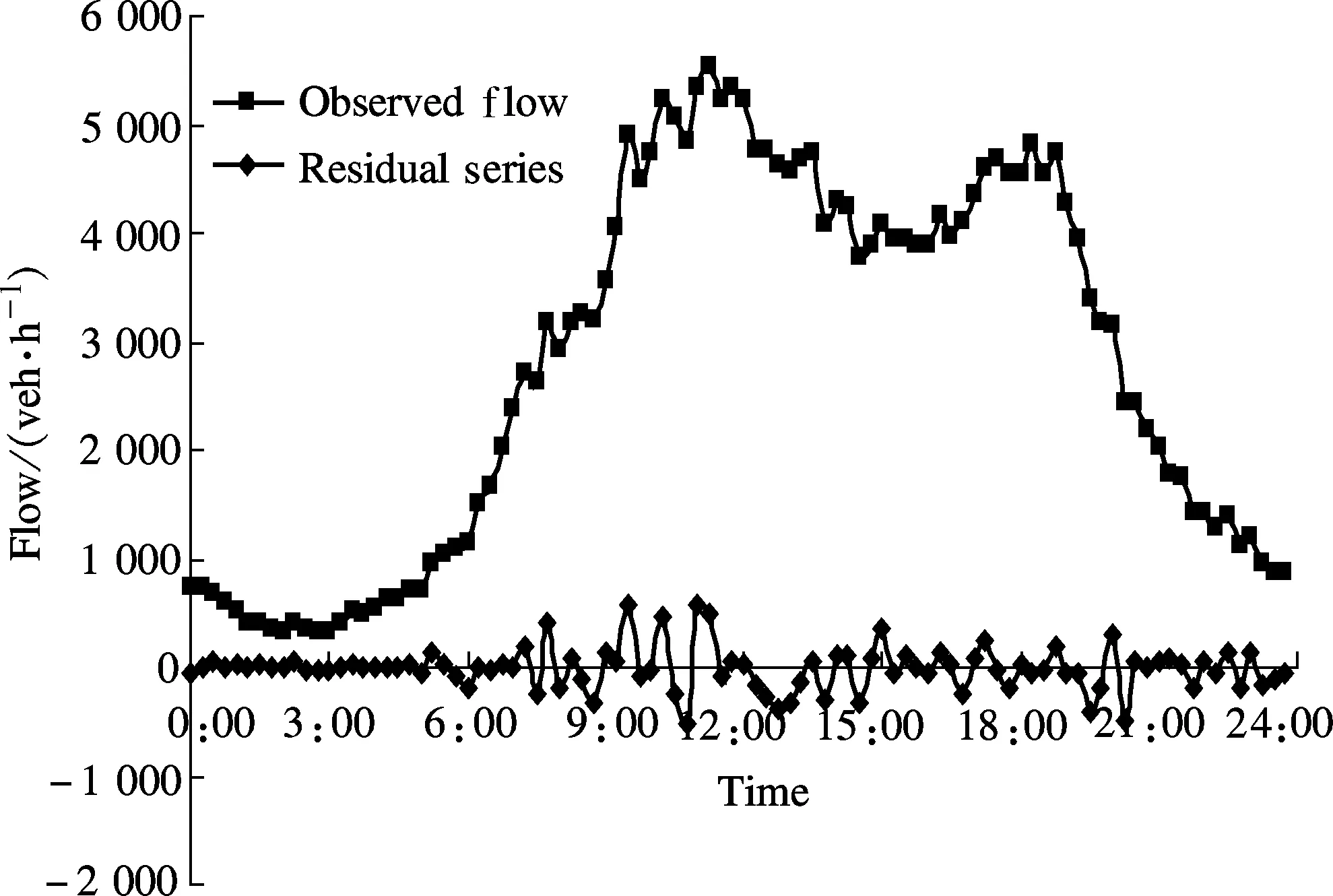
Fig.1 Traffic flow heteroscedasticity demonstration
From Fig.1, we can see that the residual series is scattered around thex-axis while the ranges of the scattering are different for different times of the day; i.e., the residuals scatter more widely for high level traffic in the daytime. This information indicates that certain measures should be taken to handle the added uncertainty for peak hour traffic when developing advanced traffic management and control systems. As mentioned previously, the heteroscedasticity is important for developing ITS applications, and Guo et al.[6]showed that this heteroscedasticity is universal across many sites for a single 15 min aggregation interval. In this paper, we will show that this heteroscedasticity is also significant across different aggregation intervals.
1.4 Heteroscedasticity test
The heteroscedasticity test will be performed on the residual series after the autocorrelation structure is removed from the traffic flow series. Based on the residual series, the tests used in this paper include the portmanteau Q-test and the Lagrange multiplier (LM) test, which have the ability of testing the presence of nonlinear effects (such as GARCH effects) in the residuals. Note that the Q-test and the LM test are among many tests that can be selected for performing the heteroscedasticity test, and these two tests are selected in this paper due to their ready implementation and application through commercial software, i.e., SAS PROC AUTOREG. For ARIMA modeling, many off-the-shelf commercial software packages have been developed and in this paper, this SAS PROC AUTOREG is applied to test the heteroscedasticity in the residual series.
2 Data Description
2.1 Data collection
The traffic flow data used in this paper was collected from the MIDAS system installed for the motorway of M25 around London, the United Kingdom. M25 was initially built for servicing the through traffic across London, while over the years, M25 gradually merged into the urban transportation system, servicing many local trips and causing serious congestion issues on M25. Under this circumstance, the MIDAS system was developed for battling this situation. Using the MIDAS, traffic data including traffic volume, speed, occupancy, etc. was continuously registered over traffic detectors installed along the motorway. In this paper, traffic flow data collected from the station 4762a is used. The time range of the data is from Jan 1, 2002, to Dec 31, 2002; i.e., the whole year traffic flow data is used in this paper.
2.2 Data aggregation
The purpose of this paper is to investigate the effect of aggregation intervals on the traffic flow heteroscedasticity. Therefore, an important step is to aggregate the traffic flow data over multiple aggregation intervals. In this paper, altogether 30 aggregation intervals are used, i.e., aggregation intervals starting from 1 to 30 min with 1 min increment. Note that the aggregation of traffic flow data follows the rule proposed by Edie[13]and the aggregation operation is carried out using SAS PROC EXPAND, through which the aggregation rule can be easily implemented. The traffic flow data aggregated at 1 min interval are shown in Fig.2. As can be seen that the seasonal pattern can be identified for this 1 min traffic flow data series, which is an important phenomenon that should be handled. In addition, this seasonal pattern also exits in traffic flow series aggregated over other aggregation intervals.

Fig.2 Traffic flow series demonstration (partial data aggregated at 1 min interval)
3 Empirical Results
In this section, the empirical results will be shown, including the ARIMA modeling results and the results of the heteroscedasticity test over multiple traffic flow series aggregated at different aggregation intervals.
3.1 ARIMA modeling results
The purpose of ARIMA modeling is to capture and remove the first-order moment of the traffic flow series and hence generate the residuals for the heteroscedasticity test. Note that we have 30 traffic flow series corresponding to 30 aggregation intervals; therefore, we will have 30 identified and estimated ARIMA models.
As mentioned previously, the ARIMA model can be processed through the steps of identification, estimation, and diagnostic check. In this paper, in the model identification step, the seasonal pattern is first handled by seasonal differencing. As identified in Ref.[14], a weekly pattern can be used. Taking the 15 min aggregation interval as an example, a weekly pattern will have 24 (h/d)×4(data point/h)×7(d)=672 data points. Therefore, for removing the seasonal effects, two traffic flow data points at a distance of 672 aggregation intervals are differenced; i.e., the seasonal differencing order is 672. After seasonal differencing, the differenced series are used to identify the orders of ARIMA.
Using PROC ARIMA, the orders of the ARIMA model for all the 30 traffic flow series are shown in Tab.1.
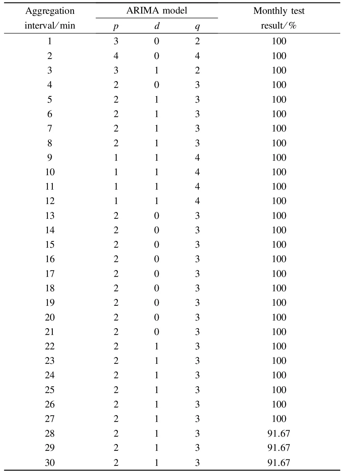
Tab.1 ARIMA modeling and heteroscedasticity test results
After selecting these orders, the ARIMA models are estimated using the maximum likelihood method and the residuals are computed using the estimated parameters. Then, in the final model diagnostic check step, the selected models and estimated parameters are validated by checking the characteristics of the residual series. According to the ARIMA modeling theory, the residual series should be white noise or the autocorrelations in the residuals are trivial, indicating that the autocorrelation structure has been adequately removed. In this paper, the autocorrelations in all the 30 residual series are trivial, indicating the adequacy of selecting the identified ARIMA models.
3.2 Heteroscedasticity test results
Based on the obtained residual series, the heteroscedasticity test results are presented as follows. In the whole series test, for all the aggregation intervals, the two heteroscedasticity tests are applied on the entire residual series with thep-values of the two test statistics less than 0.000 1, showing that for all the 30 residual series the traffic flow series are heteroscedastic.
For the monthly test, the results are also shown in Tab.1. For each aggregation interval, the entire series is first broken into monthly series, and each monthly series is tested separately. Then the percentage of the heteroscedastic monthly residual series is computed as the test results. We can see that except for the aggregation intervals of 28, 29, and 30 min that have 91.67% heteroscedastic monthly residual series, and the remaining aggregation intervals have 100% heteroscedastic monthly residual series, indicating that traffic flow series are heteroscedastic at the monthly level for these aggregation intervals. The test results indicate that the longer aggregation interval can cancel out the noise in traffic flow data and hence reduce the heteroscedasticity in traffic flow.
4 Conclusions
Considering the importance of reliability in many ITS applications, the uncertainty analysis has received increasing attention from transportation research communities. In this direction, the traffic flow heteroscedasticity test and modeling play an essential role. Previous studies have shown that traffic flow is heteroscedastic across stations for a certain data aggregation interval, and in this paper we investigate the effects of multiple aggregation intervals on traffic heteroscedasticity. Using real-world traffic flow data, the following two conclusions can be drawn as follows:
1) Traffic flow is heteroscedastic across multiple intervals ranging from 1 to 30 min at 1 min increment.
2) Longer aggregation intervals can cancel out the noise in the traffic flow data and hence reduce the heteroscedasticity in traffic flow series.
Based on the above conclusions together with the previous investigations, heteroscedasticity can be claimed to be universal for traffic flow data both temporally and spatially, and considerations should be taken to improve the reliability or robustness of ITS-related traffic management and control applications.
[1]Karlaftis M G, Vlahogianni E I. Memory properties and fractional integration in transportation time series [J].TransportationResearchPartC, 2009,17(4): 444-453.
[2]Guo J H, Williams B M. Real time short term traffic speed level forecasting and uncertainty quantification using layered Kalman filters [J].TransportationResearchRecord, 2010,2175: 28-37.
[3]Sohn K, Kim D. Statistical model for forecasting link travel time variability [J].ASCEJournalofTransportationEngineering, 2009,135(7): 440-453.
[4]Yang M L, Liu Y G, You Z S. The reliability of travel time forecasting [J].IEEETransactionsonIntelligentTransportationSystems, 2010,11(1): 162-171.
[5]Tsekeris T, Stathopoulos A. Short-term prediction of urban traffic variability: stochastic volatility modeling approach [J].ASCEJournalofTransportationEngineering, 2010,136(7): 606-613.
[6]Guo J H, Huang W, Williams B M. Integrated heteroscedasticity test for vehicular traffic condition series [J].ASCEJournalofTransportationEngineering, 2012,138(9): 1161-1170.
[7]Guo J H, Williams B M, Smith B L. Data collection time interval for stochastic short-term traffic flow forecasting [J].TransportationResearchRecord, 2008,2024: 18-26.
[8]Smith B L, Ulmer J M. Freeway traffic flow rate measurement: investigation into impact of measurement time interval [J].ASCEJournalofTransportationEngineering, 2003,129(3): 223-229.
[9]Guo J H, Huang W, Wei Y, et al. Effect of time interval on speed estimation using single loop detectors [J].KSCEJournalofCivilEngineering, 2013,17(5): 1130-1138.
[10]TRB. Highway capacity manual 2000 [R].Washington: Transportation Research Board, 2000.
[11]Box G E P, Jenkins G M, Reinsel G C.Timeseriesanalysis:forecastingandcontrol[M]. 3rd ed. Upper Saddle River, NJ,USA: Prentice-Hall, 1994.
[12]SAS Institute, Inc.SASOnlineDocversion8 [M]. Cary, NC, USA: SAS Institute, 2000.
[13]Edie L C. Discussion of traffic stream measurements and definitions [C]//Procof2ndInternationalSymposiumontheTheoryofTraffic. Paris, France, 1963: 139-154.
[14]Williams B M, Hoel L A. Modeling and forecasting vehicular traffic flow as a seasonal ARIMA process: theoretical basis and empirical results [J].ASCEJournalofTransportationEngineering, 2003,129(6): 664-672.
 Journal of Southeast University(English Edition)2013年4期
- Journal of Southeast University(English Edition)的其它文章
- Improvement of pump-probe optical measurement technique using double moving stages
- Application of neural network merging model in dam deformation analysis
- Elastoplastic response of functionally graded cemented carbidesdue to thermal loading
- Mechanical analysis of transmission lines based on linear sliding cable element
- Annoyance-type speech emotion detection in working environment
- Improvement of pump-probe optical measurement technique using double moving stages