
A random walk simulation of scalar mixing in flows through submerged vegetations*
2014-06-01 12:30LIANGDongfang梁东方
水动力学研究与进展 B辑 2014年3期
LIANG Dongfang (梁东方)
MOE Key Laboratory of Hydrodynamics, School of Naval Architecture, Ocean and Civil Engineering, Shanghai Jiao Tong University, Shanghai 200240, China
Department of Engineering, University of Cambridge, Cambridge, UK, E-mail: d.liang@sjtu.edu.cn
WU Xuefei
Department of Engineering, University of Cambridge, Cambridge, UK
A random walk simulation of scalar mixing in flows through submerged vegetations*
LIANG Dongfang (梁东方)
MOE Key Laboratory of Hydrodynamics, School of Naval Architecture, Ocean and Civil Engineering, Shanghai Jiao Tong University, Shanghai 200240, China
Department of Engineering, University of Cambridge, Cambridge, UK, E-mail: d.liang@sjtu.edu.cn
WU Xuefei
Department of Engineering, University of Cambridge, Cambridge, UK
(Received March 27, 2014, Revised April 30, 2014)
The scalar transport phenomena in vertical two-dimensional flows are studied using the random walk method. The established Lagrangian model is first applied to study the idealized longitudinal dispersion in open channels, before being used to investigate the scalar mixing characteristics of the flows through submerged vegetations. The longitudinal dispersion coefficients of the fully-developed boundary layer flows, with and without vegetations, are calculated based on the positions of the particles. A convenient way of incorporating the effects of vegetations is proposed, where all the flow parameters are regarded to be continually distributed over the depth. The simulation results show high accuracy of the developed random walk method, and indicate that the new method of accounting for the vegetation effects is appropriate for all the test cases considered. The predicted longitudinal dispersion coefficients agree well with the measurements. The merit of the new method is highlighted by its simplicity and efficiency in comparison with the conventional method that assumes the discontinuous distribution of the flow parameters over the depth.
random walk, longitudinal dispersion, submerged vegetations, scalar mixing
Introduction
Scalar transport phenomena in fluid have been studied by many researchers since the middle of the last century. To quantitatively analyze the transport of pollutants in shear layers, the longitudinal dispersion coefficient is often used to represent the mixing rate, which has become a key parameter in water-quality modeling. The dispersion coefficient is dependent on the velocity profile and transverse diffusion of the flow. Analytical solutions of the dispersion process have been obtained under several classic flow conditions, e.g., uniform open channel flows and pipe flows.
However, the idealised conditions in these classic analyses do not hold true in most natural aquatic systems, for which the presence of secondary flows andvegetations is important. Many studies have shown that aquatic vegetation is crucial to the water quality, since it is not only an indicator, but also a contributor to the level of the wellbeing of water. Studies on the vegetated flow generally categorise the vegetation into emergent and submerged types. Nepf et al.[1]proved that, for the emergent case, the production of turbulence is dominated by the stem wakes rather than by the bottom-boundary shear. In the flows with the submerged vegetation, Ghisalberti and Nepf[2]showed that the vertical mass transport is dominated by the coherent vortices of the vegetated shear layers. The vertical turbulent diffusivity is directly proportional to the shear and thickness of the layer. With the knowledge about the vertical diffusivity of different regions in the vegetated flow and the flow velocity profile, the process of material mixing could be simulated. In rivers and estuaries, the drag induced by the submerged vegetation leads to the velocity profiles and the transverse diffusion coefficients that differ significantly from those in a conventional fully-developed boundary layer[2], invalidating the assumptions behind Elder’sanalysis. Therefore, in such cases, a more complex analysis of the dispersion process is required.
Many numerical methods for pollutant transport phenomena have been developed for various contaminants in a variety of aquatic environments. Generally, these methods can be classified into either Eulerian or Lagrangian methods. By now, most of the research has been conducted using Eulerian methods[3,4]. Some hydrodynamic investigations include the impact of vegetation through adding drag resistance and increasing bottom roughness[5-7]. Based on the force balance in a control volume, the analytical solution of the streamwise velocity distribution can be derived accordingly. In the study of scalar mixing, the Lagrangian approach is often regarded as more accurate, although being more computationally expensive. It is also commonly called the random-walk method. In this method, the pollutant cloud is represented by a large number of discrete massless particles that are released into the flow as indicators and are tracked independently. Hence, by definition, the Lagrangian approach is perfectly conservative and free from artificial diffusion near the steep concentration gradients. Furthermore, the computation is limited to the regions that the pollutant reaches, while the computation in the Eulerian methods always needs to cover the entire domain. This paper applies the random walk method to study the longitudinal dispersion processes in open channel flows in the presence of submerged vegetations.
1. Random walk method and longtitudinal dispersion without vegetation
As was mentioned above, the random walk method is an alternative to the conventional Eulerian simulation of mass transport phenomenon in flows. It tracks the motion of discrete particles. In this paper, we limit our discussion to the vertical two-dimensional case. Gardiner[8]has proved that the particle displacement, whose two components are Δxand Δy, in each time step is composed of two parts as shown in Eqs.(1a), (1b)
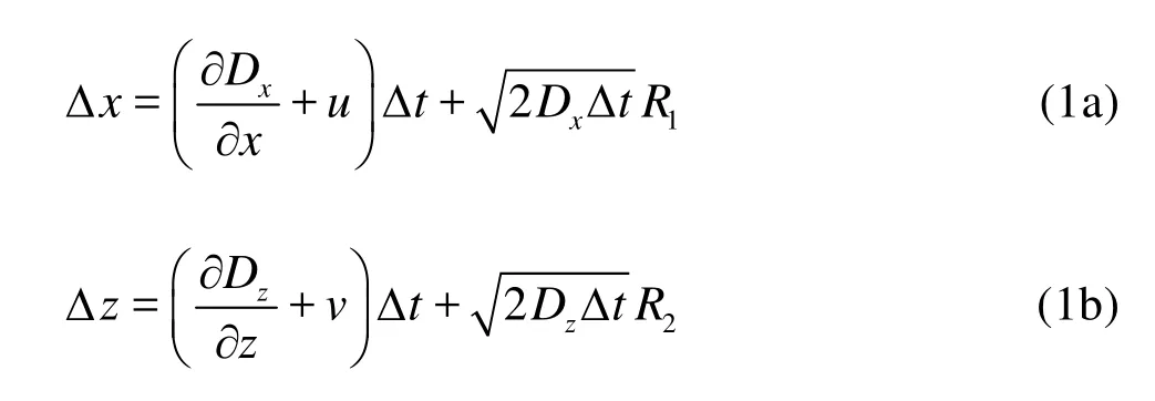
where the first term on the right hand side represents the deterministic forces acting to change the particle position over time, the stochastic part relies on the second term, which represents the rapidly changing forces,DxandDzare the diffusion coefficients in the longitudinal and vertical directions, respectively,uandvare the longitudinal and vertical velocities, respectively,R1andR2are two independent random variables with standard Gaussian distribution[9]. More detailed derivations of the equations can be referred to Dimou[10].
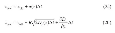
For simplicity while without much loss in accuracy, an assumption of constant water depth,h, is made in this study. Furthermore, in a shear flow, advection in longitudinal direction along thexaxis and diffusion in vertical direction along thezaxis dominate the mass transport in the flow. According to Taylor’s assumption, the longitudinal diffusion in thex-direction as well as the drift component in thez-direction are both negligible. Hence, a simplified version of Eq.(1) can be adopted to update the particle positions in open channel flows with no vertical velocity component where the mean horizontal flow velocity only varies in the vertical direction. Similarly, the turbulent diffusion coefficientDzis a function of the vertical position only in this study.
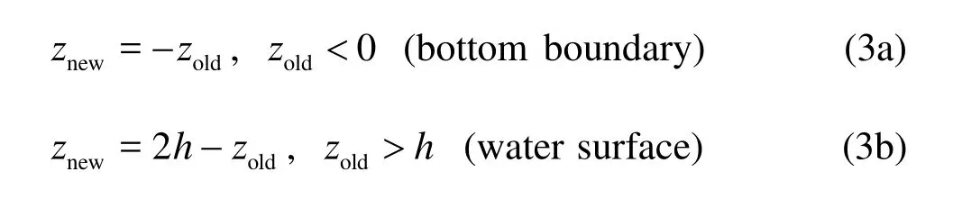
Inside the calculation domain, the particles follow a “random walk” path with the flow, as dictated by the above equation. At boundaries, however, special treatments are needed to prevent them from crossing the boundaries. The water surface and the channel bottom are regarded to act as reflective mirrors. Particles crossing them would be reflected back into the domain. In this study, the bed always coincides withz=0, and the water surface always coincides withz=h. Hence, the boundary conditions can be expressed as
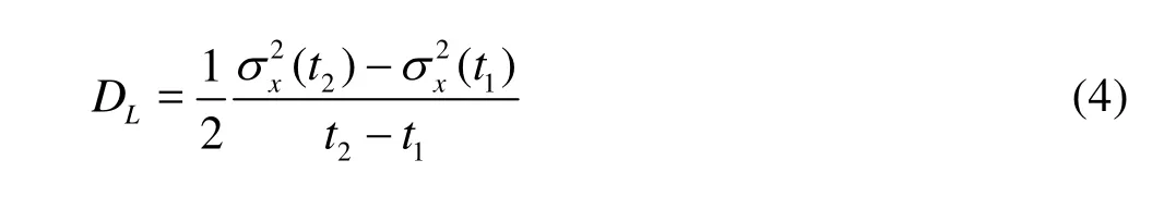
According to the above procedures, the position of every particle at every time step can be simulated. By analyzing the statistics of the positions of a large number of particles, the longitudinal dispersion coefficientDLcould be determined. After a certain time since the release of the particle ensemble, known as the Fickian time, the standard deviation of particles’positions in the longitudinal direction increases linearly with time, indicating thatDLconverges to a constant. As a measure of the spatially-averaged spreading rate of a tracer cloud,DLcan be calculated ac-cording to the time change of the longitudinal variance of the particle ensemble
To verify the newly-established model, the idealised case in the open channel flow without any vegetation was first tested to see whether the results agree well with the analytical solutions. Figure 1 is the random-walk model results for this case, whose velocity profile over the depth is determined by the logarithmic law
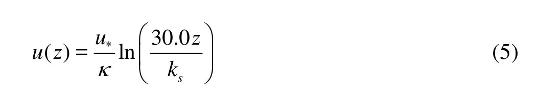
where the friction velocityu*=0.01 m/s, the von Kármán constantκ=0.41, and roughness heightks= 0.01 m. In general, the smaller the time step is, the more accurate and stable the simulation will be, although the more computational expensive it might be. At present, time step is set to be 0.05 s for open channel flows without vegetation. The water depth is assumed to be 1 m and remains constant, and whent= 0 s, 100 000 particles are released uniformly atx=0 over the depth. Figure 1 illustrates the particle distributions and histograms at different times along thexdirection.
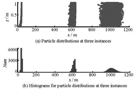
Fig.1 Particle distributions and histograms in turbulent open channel flow
We compared the simulation results with the analytical solutions for this classic case. Beyond the Fickian time, the distributions of the particles becomes Gaussian and the concentration profiles in the longitudinal direction agree well with the analytical solutions, as shown in Fig.2. The Fickian time is the time after which the longitudinal dispersion coefficientDLconverges to a constant, and it will be discussed in detail later. The Fickian time is calculated to be 585 s for this problem. In Fig.2, the black lines are calculated directly from the analytical solutions, given the flow and initial conditions mentioned above. Assume unit mass for one particle, then the total mass that are released att=0 equals to the number of particles. Meanwhile the gray bars, which represent calculated concentration in each volume of water body, are calculated by the number of particles in the column divide the volume of the column.
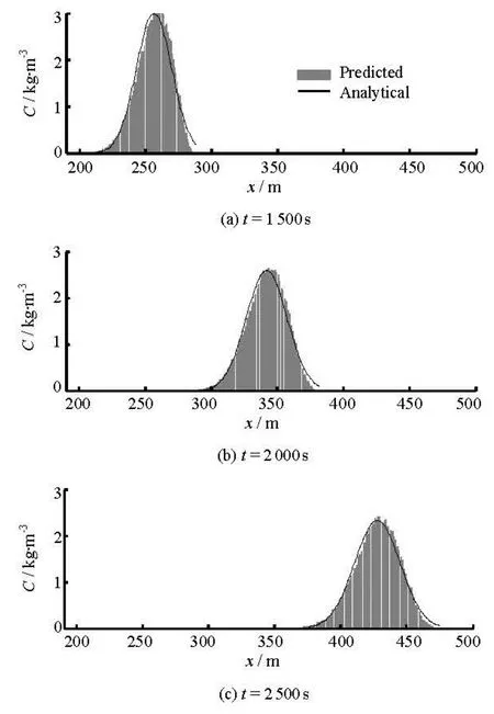
Fig.2 Comparison between the computed and analytical concentrations
2. Schematisation of the flow through vegetation
To apply the random walk model to the vegetated open channel flows, specific knowledge is needed concerning the velocity profile as well as the diffusion coefficient profile, which are influenced significantly by the vegetation. Several experiments have been conducted to study the vegetated flow in the laboratories.
In Ghisalberti and Nepf[2]and Murphy[11], the experiments were taken in a 24 m long, 0.38 m wide and 0.58 m deep, glass-walled recirculating flume. The model plant canopy consisted of rigid cylinders with a diameterd=0.006 m, which were inserted to the bed in a random configuration. The canopy density,ad, was varied between 0.015 and 0.048, whereadonated the frontal area per unit volume of the entire canopy. The canopy height was fixed either 0.14 m or0.07 m. A summary of the typical experimental conditions and the measured vegetated shear flow parameters, which will be used later in the random walk simulations, are listed in Table 1.
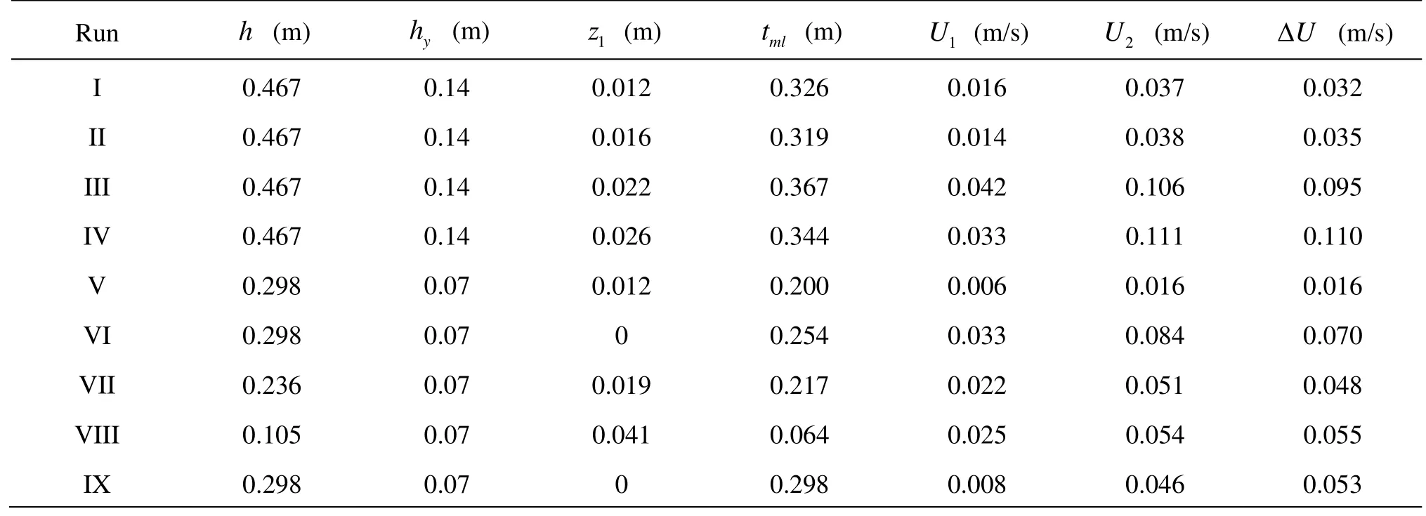
Table 1 Computational conditions of the nine cases
In Table 1,handhyrepresent water depth and vegetation height, respectively,z1is the depth of wake zone near the bottom,tmlis the thickness of the mixing layer,U1andU2are the average velocities in the lower and upper water columns, respectively. ΔUis the shear velocity across the middle layer, which is given by the experiments with a magnitude ofU2-U1.
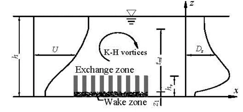
Fig.3 The structure of the velocity and diffusivity profiles
Corresponding to the data in Table 1, the key flow features of the flow through submerged vegetation are illustrated in Fig.3[2,11]. The vegetation is illustrated by the black bars. The vertical velocity profile, as seen in the left part of Fig.3, is divided into three zones. The wake zone is of the thicknessz1, lying at the bottom of the vegetation. Fluid flows slowly in this zone due to the drag of vegetations. The second zone is in the middle with a thicknesstml, where the flow is dominated by the Kelvin–Helmholtz (K-H) vortices and the velocity increases gradually with depth. On top of this middle zone lies the third zone, with the largest velocity. The velocity difference ΔUis proportional to the rotating velocity of the K-H vortices.tmlLikewise, can be comprehended as the length scale of the K-H vortices. The diffusivity distribution over the water depth, as illustrated in the right part of Fig.3 is supported by the experimental data[2].

Fig.4 The “two-box” velocity and diffusivity profiles
To implement the two-dimensional random walk method, Murphy[11]devised a two-box profile to represent the distributions of the velocity and diffusivity, as illustrated in Fig.4, which is widely used in the literature[12,13]to represent the flow structures. The height of the submerged vegetation is chosen to be the separatrix of the two boxes. The constant values in the upper and lower boxes are derived by averaging the variations in the two parts respectively. The discontinuities in the middle complicate the random walk simulations. One special treatment to address the discontinuities is as follows. Due to the discontinuous velocity atz=hv, particles need to cross the interface in requiresDz(z) to be differentiable. To handle the diffusivity discontinuity atz=hy, a semi-reflecting two steps, and thus the original time step should be split into two parts. Besides, the application of Eq.(1) boundary has been proposed[11,13]. Therefore, the simple concept of this two-box model does not lead to a numerical implementation. Moreover, it is obvious by comparing Fig.3 and Fig.4 that the two-box model gives a very crude approximation of the measured ve-locity and diffusivity profiles.
In order to overcome the problems associated with the two-box model, a refined three-zone model is proposed in this study to represent the vegetated flows, which is a better reflection of the true distributions of velocity and diffusivity. The three zones include one zone within the canopy, one zone above the canopy and one zone in between as a transition region. Constant velocities,U1andU2are assumed at the lower and upper zones, respectively. Likewise, the diffusion coefficients,Dz1andDz2, are regarded as constants in the slow and fast zones. The velocity and the diffusion coefficient in the transition zone are assumed as follows.
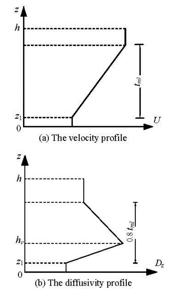
Fig.5 The three-layer velocity and diffusivity profiles in the refined model
The velocity in the transition zone needs to connect the two constants in the upper and lower zones. A linear function is proposed between the fast and slow zones in this paper, as shown in Fig.5(a). The real middle velocity profile follows a hyperbolic tangent shape[14], but this linear simplification was proved to be acceptable in accuracy with higher computational efficiency. It also keeps the same flow rate as the hyperbolically-distributed velocity profile.
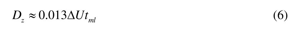
In the “wake zone”, the diffusivity is constant. The diffusivity in this zone is equivalent to that with emergent canopies and is sensitive to the diameter of the plant, density of the vegetation, and the flow velocity in the zone. Nepf et al.[1]related the value of this diffusivity to the stem Reynolds number and the stem area density. In the upper layer,z>(z1+0.8tml), there is a secondary circulation presumed to exist above the shear layer. In this region, the diffusivityDzdepends on the size of the K-H vortices below and their characteristic rotational speed, as demonstrated in Eq.(6)
In the middle layer, the turbulent diffusivity peaks near the top of the canopy. For various plant densities, the peakDz/(ΔU·tml) remains roughly equal to 0.032. The diffusivity is assumed to linearly increase from the bottom value to the peak value at the top of the canopy, before linearly decrease to the value in the upper zone, as shown in Fig.5(b). Such assumption is corroborated by experimental data, asillustrated in the right part of Fig.3.

Fig.6 The longitudinal dispersion coefficients versus time for different numbers (Run III in Table 1)
3. Longitudinal dispersion in the flow through vegetation
3.1Effect of number of particles
With the refined velocity and diffusivity profiles, which are both continuous, the “random walk” method could be applied to the flows with submerged vegetation in the same way as that demonstrated in the previous section. Initially, all the particles are released at the top of the canopy as in the experiments. The time step is chosen to be 0.05 s. First of all, the impact from the number of particles used in simulation is studied. Figure 6 shows the evolution of the instantaneous dispersion coefficient with time,D=0.5∂σ2/
Lx∂t. As was expected, the more particles used, the more stable the result is. This trend applies to all the flow conditions considered in Table 1, while only one of them is selected in the demonstration in Fig.6. On the other hand, the computational cost increases with the number of particles. For the random walk method, it is known that the amount of calculation increases li-nearly with the number of particles, because the time step can be decoupled with the number of particles. In the following simulations, we set 100 000 particles for all the runs.
3.2Fickian time and longitudinal dispersion coefficient
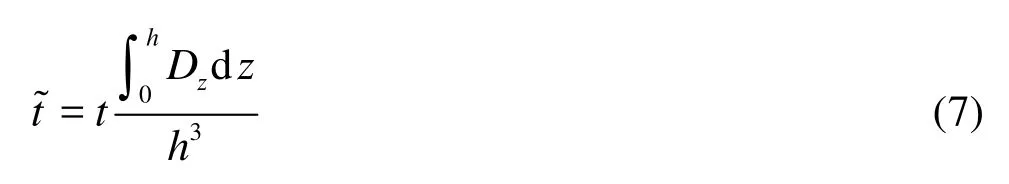
whereis a dimensionless time scale for cross-sectional mixing. Fischer takes the minimum value ofto be 0.4. However,should be bigger than this to take into consideration of the impact from vegetation, especially the reduced diffusion in the wake zone. Based on Eq.(7), the Fickian time for each case is estimated in Table 2.
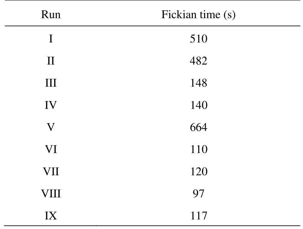
Table 2 Fickian times for nine cases by assuming the Fickian time scale to be 0.4
From Table 2, a fairly conservative time scale for obtaining a stable linear increase ofcan be carefully determined. After that time, the calculated longitudinal dispersion coefficientDLwill converge to a constant value, as shown for the representative three cases in Fig.7, where the observed longitudinal coefficients and the Fickian times are labeled as solid horizontal lines and dashed vertical lines respectively.
The estimation of the Fickian time agrees well with the simulation results. The stabilized longitudinal coefficients were compared with the observed data from Murphy[11], with an average error of 15.3%, as shown in Table 3 and Fig.8.
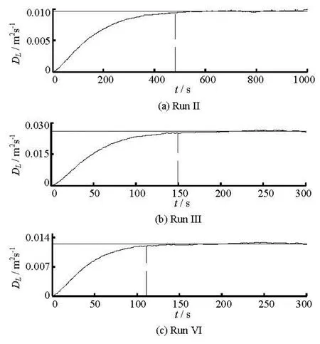
Fig.7 Time series of the longitudinal dispersion coefficient (the curve line) compared with the observed value (the straight line), with Fickian time labeled by the vertical dashed line
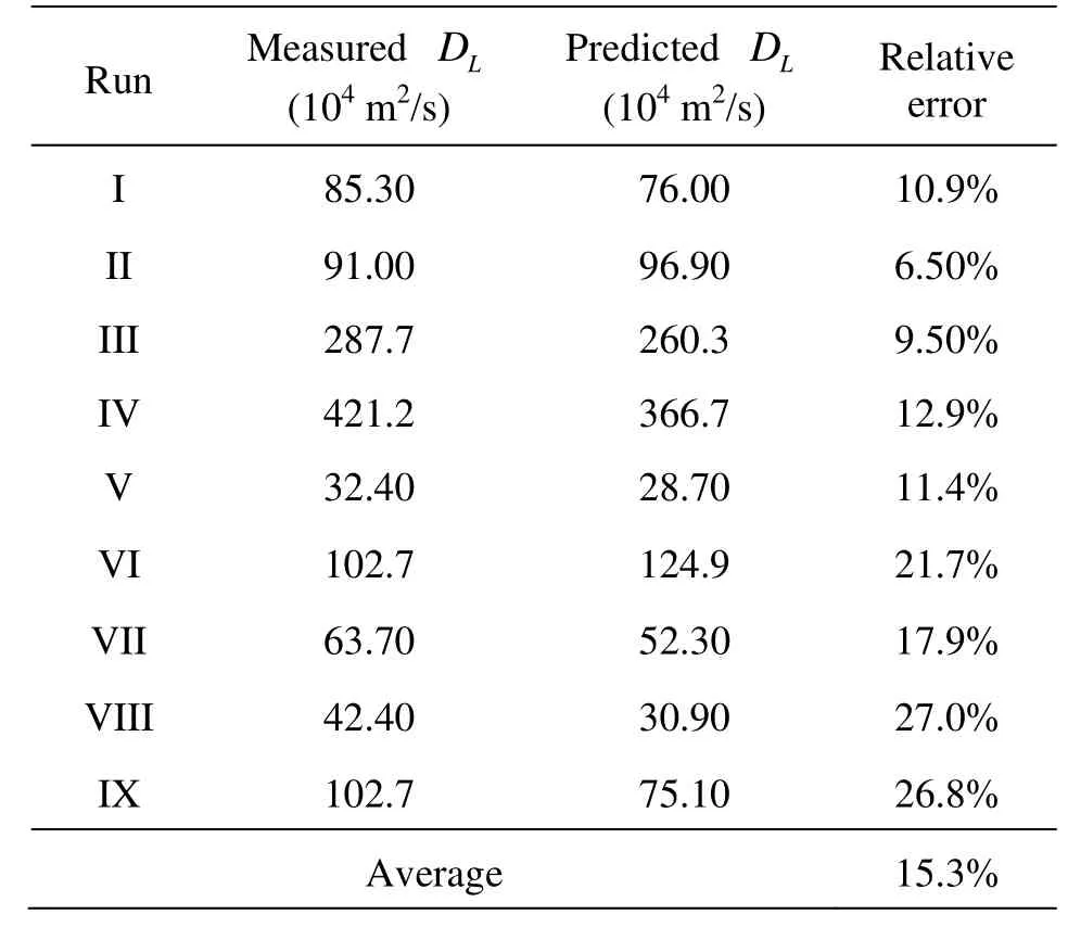
Table 3 Comparison between the observed and predictedDL
3.3Sensitivity analyses
The algorithm of the random walk model in this paper requires the determination of several key flow parameters, among which are the water depth, the vegetation height, the thickness of wake zone at the bottom, the thickness of the mixing layer, the constant velocities in the lower and upper zones, and the shear velocity across the middle layer. In the above simulations, these data are simply obtained from the experiments by Ghisalberti and Nepf[2]and Murphy[11], as presented in Table 1. The water depth and vegetation height can be accurately determined and the measure-ments ofU1andU2can also be quite accurate, so these values are fixed in the sensitivity analysis. The remaining parameters include the thickness of the wake zone, the thickness of the mixing layer and the total velocity difference across the middle layer, which are the focus of the current sensitivity analyses. They are increased/decreased by 10% to examine how the computed longitudinal coefficients are sensitive to these changes.
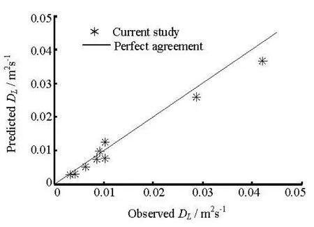
Fig.8 Comparison between the measured and predictedDL
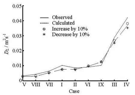
Fig.9 Sensitivity analysis of the depth of wake zone
Both the flow and the diffusion are weak in the wake zone, making it similar to the dead zone[15]. When the thickness of the wake zone increases from
z1to, the upper and lower constants of diffusivity as well as the maximum of diffusivity are unchanged. On the other hand, an increasedz1leads to larger diffusivity in the upper half of the middle zone, while results in smaller diffusivity in the lower half in a greater degree. Hence the increase ofz1leads to an overall decrease of the diffusivity. For wide open channel, the analytical solution shows that the longitudinal dispersion coefficient is inversely proportional to the vertical diffusivity. In analogy, we expect the overall decrease in diffusivity leads to an increase in longitudinal dispersion in vegetated flows. In the case of velocity, the impact of a thicker wake zone is more complicated. In order to preserve the same flow rate, larger velocities have to be applied in the middle and upper zones. As a result, an increasedz1is accompanied by a steeper gradient of velocity distribution, which is also expected to increase the longitudinal dispersion coefficient. These analyses are proved by Fig.9, where the longitudinal dispersion coefficient is larger ifz1is increased by 10% for all the cases.
Similar analyses are taken to examine the impact oftml. To conserve the flow rate, the velocity gradient needs to increase slightly. At the same time, the diffusivity increases along the middle zone, due to the thicker mixing layer. The stronger shearing of the incoming flow and the larger vertical diffusivity pose opposite influence on the magnitude of the dispersion coefficient. Therefore, the increase intmlshould lead to a decrease in the longitudinal dispersion coefficient, as evidenced in Fig.10.
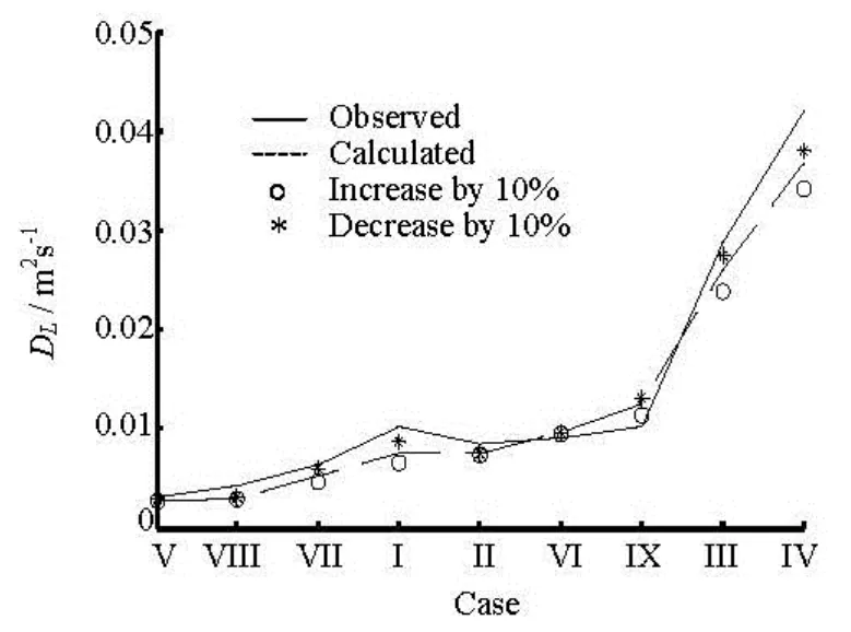
Fig.10 Sensitivity analysis of the thickness of the mixing layer
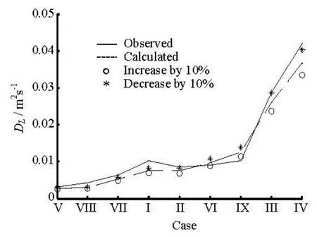
Fig.11 Sensitivity analysis of the shear velocity across the middle layer
ΔUdoes not influence the velocity profile in this simulation. However, its impact on the diffusivity profile is the largest among the three analyzed parameters. Based on Eq.(6), the diffusivity in the upper zone increases linearly with ΔU. In addition, a larger ΔUalso increases the maximum of diffusivity in the middle zone. Hence, the diffusivity becomes larger along the middle and upper zone. As was mentioned above, the longitudinal dispersion coefficient is inversely proportional to vertical diffusivity coefficient,thus an increased ΔUshould result in a smallerDL, as confirmed by Fig.11.
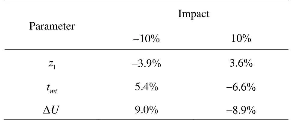
Table 4 Results of the sensitivity analyses
To sum up, Table 4 lists the impact of these three parameters on the dispersion coefficient. The percentages of the relative changes are the averages among all the nine runs.DLincreases with the increase ofz1, the decrease oftml, and the decrease of ΔU. Among them,z1has the least influence, and ΔUhas the largest influence on the computed dispersion coefficients.
4. Conclusion
The random-walk model established in this paper has been shown to accurately predict the longitudinal dispersion coefficients in the flows with and without submerged vegetations. With the presence of vegetations, the refined model in this paper adopts the threezone continuous velocity and diffusivity profiles, which leads to a better representation of the measured experimental profiles than the method with the twobox discontinuous profiles used by previous researchers[11-13]. Meanwhile, these continuous profiles improve the robustness of the random-walk model by eliminating the necessity for the complicated “semireflective” boundary between the two discontinuous zones. With this refined random walk model, the dispersion processes in nine flow conditions were simulated, and good agreements with the measurements were achieved. Sensitivity analyses have also been conducted, which involve the depth of wake zone, the thickness of the mixing layer and the shear velocity across the middle layer. These three parameters are selected because they are obtained indirectly in the experiments and thus the main sources of uncertainties. Through increasing and decreasing their values by 10%, their impacts on the calculated longitudinal dispersion coefficientDLwere illustrated. The shear velocity is found to play the most crucial role in the dispersion process, followed by the thickness of the mixing layer and then the depth of the wake zone.
Acknowledgements
This work was supported by the Non-profit Industry Financial Program of the Ministry of Water Resources (Grant No. 201401027), and the China Scholarship Council.
[1] NEPF H. M., SULLIVAN J. A. and ZAVISTOSKI R. A. A model for diffusion within emergent vegetation[J].Limnology and Oceanography,1997, 42(8): 1735-1745.
[2] GHISALBERTI M., NEPF H. Mass transport in vegetated shear flows[J]Environmental fluid mechanics,2005, 5(6): 527-551.
[3] LIANG D., WANG X. and FALCONER R. A. et al. Solving the depth-integrated solute transport equation with a TVD-MacCormack scheme[J].Environmental modelling and Software,2010, 25(12): 1619-1629.
[4] LIANG D., WANG X. and BOCKELMANN-EVANS B. N, et al. Study on nutrient distribution and interaction with sediments in a macro-tidal estuary[J].Advances in Water Resources,2013, 52: 207-220.
[5] WANG Pei-fang, WANG Chao. Numerical model for flow through submerged vegetation regions in a shallow lake[J].Journal of Hydrodynamics,2011, 23(2): 170-178.
[6] ZHANG Jian-tao, SU Xiao-hui. Numerical model for flow motion with vegetation[J].Journal of Hydrodynamics, 2008, 20(2): 172-178.
[7] HUAI Wen-xin, CHEN Zheng-bing and HAN Jie et al. Mathematical model for the flow with submerged and emerged rigid vegetation[J].Journal of Hydrodynamics,2009, 21(5): 722-729.
[8] GARDINER C. W.Handbook of stochastic methods[M]. Berlin, Germany: Springer, 1985.
[9] HOTEIT H., MOSE R. and YOUNES A. et al. Threedimensional modeling of mass transfer in porous media using the mixed hybrid finite elements and the randomwalk methods[J].Mathematical Geology,2002, 34(4): 435-456.
[10] DIMOU K. Simulation of estuary mixing using a twodimensional random walk model[D]. Master Thesis, Cambirdge, Massachusetts, USA: Massachusetts Institute of Technology, 1989.
[11] MURPHY E. Longitudinal dispersion in vegetated flow[D]. Master Thesis, Cambirdge, Massachusetts, USA: Massachusetts Institute of Technology, 2006.
[12] GHISALBERTI M., NEPF H. M. The limited growth of vegetated shear layers[J].Water Resources Research,2004, 40(7): 1-12.
[13] ROSS O. N., SHARPLES J. Recipe for 1-D Lagrangian particle tracking models in space-varying diffusivity[J].Limnology and Oceanography Methods,2004, 2: 289-302.
[14] GHISALBERTI M., NEPF H. M. Mixing layers and coherent structures in vegetated aquatic flows[J].Journal of Geophysical Research: Oceans,2002, 107(C2): 3-1-3-11.
[15] HARVEY J. W., SAIERS J. E. and NEWLIN J. T. Solute transport and storage mechanisms in wetlands of the Everglades, south Florida[J].Water Resources Research,2005, 41(5): 1-14.
10.1016/S1001-6058(14)60039-1
* Biography: LIANG Dongfang (1975-), Male, Ph. D., Professor
- 水动力学研究与进展 B辑的其它文章
- Numerical simulation of landslide-generated impulse wave*
- Scaling of maximum probability density function of velocity increments in turbulent Rayleigh-Bénard convection*
- Dispersion in oscillatory electro-osmotic flow through a parallel-plate channel with kinetic sorptive exchange at walls*
- Evaluation of the use of surrogateLaminaria digitatain eco-hydraulic laboratory experiments*
- A numerical study on dispersion of particles from the surface of a circular cylinder placed in a gas flow using discrete vortex method*
- Numerical simulation of the aerodynamic characteristics of heavy-duty trucks through viaduct in crosswind*