Effects of the wave directionality on wave transformation*

LIU Shu-xue （柳淑学）， LI Jin-xuan （李金宣）， SUN Zhong-bin （孙忠滨）

1. State Key Laboratory of Coastal and Offshore Engineering， Dalian University of Technology， Dalian 116024，China， E-mail: liusx@dlut.edu.cn

2. River and Harbor Engineering Department， Nanjing Hydraulic Research Institute， Nanjing 210029， China

Effects of the wave directionality on wave transformation*

LIU Shu-xue （柳淑学）1， LI Jin-xuan （李金宣）1， SUN Zhong-bin （孙忠滨）2

1. State Key Laboratory of Coastal and Offshore Engineering， Dalian University of Technology， Dalian 116024，China， E-mail: liusx@dlut.edu.cn

2. River and Harbor Engineering Department， Nanjing Hydraulic Research Institute， Nanjing 210029， China

2015，27（5）:708-719

A numerical model is proposed based on the time domain solution of the Boussinesq equations using the finite element method in this paper. The typical wave diffraction through a breakwater gap is simulated to validate the numerical model. Good agreements are obtained between the numerical and experimental results. Further， the effects of the wave directionality on the wave diffraction through a breakwater gap and the wave transformation on a planar bathymetry are numerically investigated. The results show that the wave directional spreading has a significant effect on the wave diffraction and refraction. However， when the directional spreading parameter sis larger than around 40， the effects of the wave directional spreading on the wave transformation can be neglected in engineering applications.

Boussinesq equations， multi-directional waves， wave directional spreading， wave transformation

Introduction

The sea waves are multi-directional irregular waves with the wave energy distributed over a wide range of frequencies and directions. As the irregular waves propagate through a gap of breakwaters or into a shallow water， they undergo transformations due to the wave shoaling， the refraction， the diffraction and the wave-wave interactions. Thus their frequency spectrum， the directional spreading and the distributions of the wave crest may undergo changes， which is important for an accurate nearshore wave predictions，which in turn is critical for designing coastal structures.

The wave directional spreading has significant effects on wave transformations in the nearshore region.Feddersen［1］measured the wave radiation stress that drives alongshore currents， and compared it with the narrow-band approximation. It is shown that the narrow-band approximations overestimate the true radiation stress components owing to the effects of the wave directions. Also， Illc et al.［2］investigated the influences of the wave directionality on the hydrodynamics processes associated with a detached breakwater. It is found that the diffracted wave heights in the lee of the breakwater can be underestimated if the random multidirectional waves are represented by a single wave. Pujianiki and Kioka［3］studied the effect of the directional wave transformation on the sloping beach. It is shown that as the waves propagate to the coast，the directional spreading becomes narrow owing to the wave refraction effect. These studies all indicate that the wave directional spreading has a definite effect on the wave transformation， but it remains to reveal what these effects are.

Numerical models are powerful tools in estimating the wave properties in harbours or wave shoaling because of their much lower cost compared with physiccal models. The numerical models based on different equations were developed to simulate the wave transformation in coastal regions， such as the Mild slope equation （MSE） models［4，5］， the spectral wave models［6，7］， and the Boussinesq equation models［8-12］. Among these models， the Boussinesq equations due tothe inclusion of a weak nonlinearity， a dispersion and a time dependence give a better description of the wave transformation， and are widely used. The applicability of the classical Boussinesq equations is confirmed for shallow water. In recent years， efforts were made to extend the application range of the equations to greater depths by improving the dispersive properties of the equations. Typical examples can be found in Ref.［13］， Madsen and Fuhrman［9］， among others. Numerical models based on the equations are established mostly using the finite difference method. However， in view of the adaptability of the finite element method to complex domains， as would be the case in most coastal engineering problems， Li et al.［14］and Liu et al.［15］developed numerical models based on the Boussinesq equations using the finite element method.

In this paper， the numerical model is briefly described， with unstructured finite elements， and a source function method is used to generate the expected waves in the computation domain， thus prevent the wave re-reflections from the incident boundaries. It is verified by the comparisons of the numerical results and associated experimental data for the multidirectional wave diffraction through a breakwater gap. In addition， to show the effects of the wave directional spreading on the wave transformation， the multidirectional wave diffraction through a breakwater gap is numerically investigated in detail. Further， the multidirectional wave propagation over a 1:25 planar beach is simulated using the numerical model for different cases of multidirectional waves， with a narrow directional spreading up to the widest spreading.

1. Numerical model

1.1 General description of the numerical model

The numerical model based on the Boussinesq equations using the finite element method was developed by Liu et al.［15］. It was used to simulate the multidirectional focusing wave run up on a vertical surface-piercing cylinder by Sun et al.［16］. The Boussinesq equations， derived by Beji and Nadaoka［17］， are expressed as

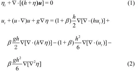
where u =（u，v）is the two-dimensional depth-averaged velocity vector，η is the water surface elevation，h=h（x，y）is the water depth as measured from the still water level，gis the gravitational acceleration. The subscriptt denotes the partial differentiation with respect to time.βis a constant. Comparing the dispersion relation of the linearized forms of Eqs.（1） and（2） with that of the linear theory，β=1/5is the best choice. The model is accurate in dispersion characteristics forkhless than 2π when β=1/5， while the linear shoaling is accurate only forkhless than π/2.

After the time derivatives in Eq.（2） are grouped together， the following two equations can be obtained

in which R=（r，s）represents the grouped time derivative terms for the two-dimensional depth-averaged velocity. The numerical solution of the original equations amounts to solve the combined equations of Eqs.（1）， （3） and （4）. The computational domain is discretized into finite elements. Since linear unstructured elements are used in the model， the nodal values of the spatial first derivatives of the surface elevationη are determined by the weighted average of the derivatives in the elements surrounding the node. The time integration is performed using the fourth order Adams-Bashforth-Moulton predictor-corrector scheme.

The calculated values ofR from Eq.（3） are then substituted back into the finite element equation corresponding to Eq.（4） to obtain the values of（u，v）at the time step（n +1）. It should be noted thatuandv are coupled in Eq.（4）， which has to be solved by an iteration scheme. Details can be found in Ref.［14］.

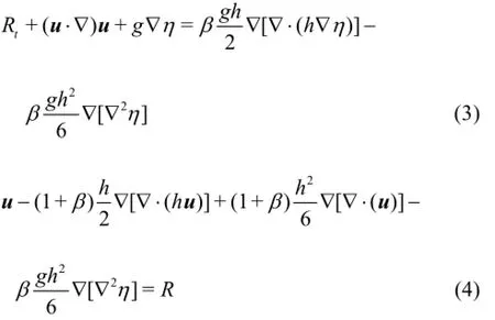
Experience with this model shows that the time interval ∆tand the element size ∆xshould satisfy the following conditions

where cwis the wave celerity andLis the local wave length. The condition （5b） can be viewed as the requirement for the density of grid points. For irregular waves， the frequency bandwidth should be determined carefully， and the highest frequency should be within the limitation of the model. Smaller elements should be used for highly non-linear waves because of the generation of higher harmonics.

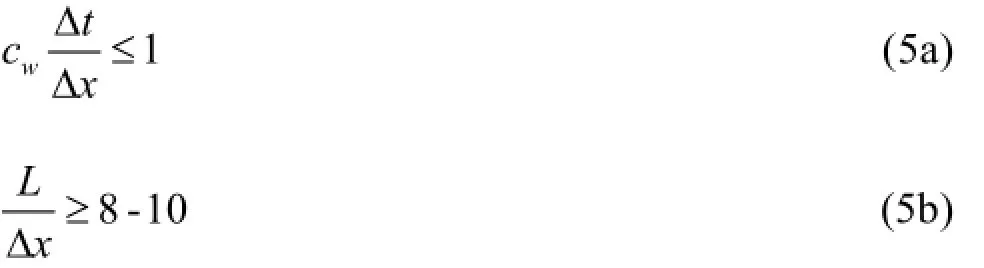
Fig.1 Computational domain for the wave diffraction through a breakwater gap

1.2 The source function method

To deal with the wave absorption of the outgoing waves from the computation domain at the incident boundary， the source function method is used （Fig.1）. In essence， the expected waves are generated in the computation domain and the outgoing waves are absorbed by some other effective methods， e.g.， the sponge layer in front of the incident boundary. To generate the expected waves in the computation domain， a pressure function Ft（x，y，t）in the source area is introduced in Eq.（2）. In the case of the constant water depth，the linearized form of Eq.（2） together with the pressure function can be written as

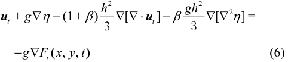
The pressure function can be expressed in the following form

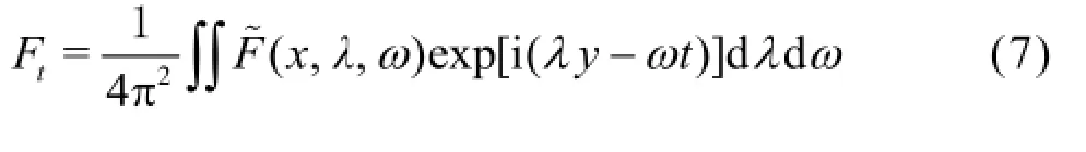
where λ=ksinθ，θis the wave direction andis in the following form

whereσis the source width and D（ω，θ）is related to the simulated wave characteristics and is expressed as

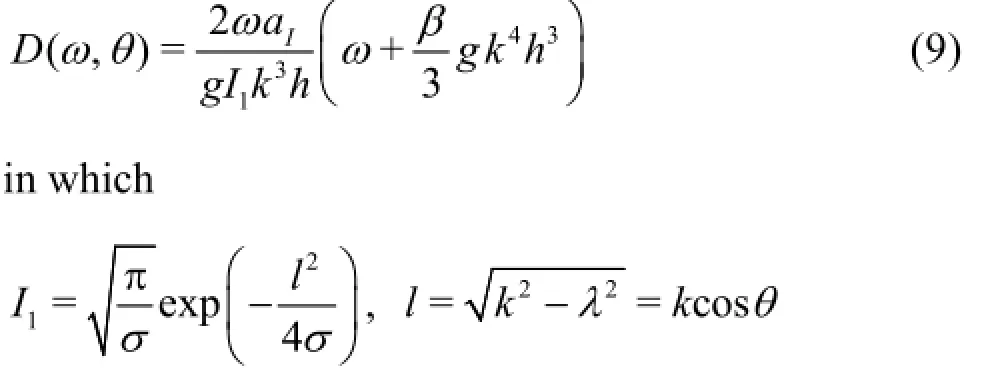
k is the wave number and aIis the incident wave amplitude.δis a constant and its typical value is in the range of 0.3-0.5 and the corresponding source function width is about 0.15-0.25 of the wave length.

1.3 Boundary conditions

Appropriate boundary conditions are needed for the numerical modelling of the wave propagation. In the following computation， three types of boundaries are considered. They are （1） the incident wave boundaries， （2） the reflective boundaries， and （3） the absorbing boundaries.

1.3.1 Incident wave boundaries

If the incident wave elevation ηIis given， the incident wave velocities can be determined by the solutions of Eqs.（1） and （2） in the linearized forms as

whereθis the wave propagation direction，ωis the wave circular frequency，kis the wave number and his the water depth. When the source function method is used， the source function can be expressed based on Eq.（7） as

where a line source at x=xsis assumed in the computation domain.

For multi-directional irregular sea waves， the incident wave elevationηIcan be modelled by a superposition of regular waves with different frequencies and propagation directions. Several methods to simulate directional sea waves were developed. In this paper， the modified double summation model is used，i.e.，

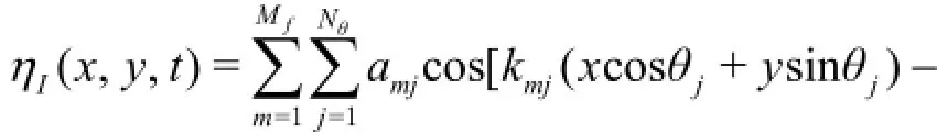
where

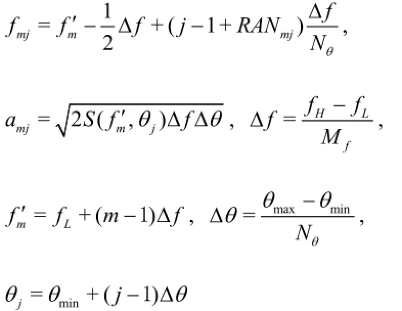
The directional spreading function G（f，θ）satisfies the following two conditions

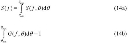
The Mitsuyasu-type spreading function is used in the following computation， i.e.，

where θ0is the principal wave direction and G0is a constant introduced to satisfy the condition （14b）.s is called the directional spreading parameter or the wave directional concentration parameter. Althoughs is a function of the wave frequency for real waves， the dependence of the directional spreading concentration parameters on the frequency is neglected to simply the calculations because the studies in this paper are focused on the effect of the directional spreading on the wave transformation.

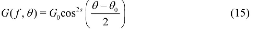
Combining Eqs.（10） and （12）， the incident velocities uI（x，y，t ）and vI（x，y，t）can be obtained using the superposition method. Similar to Eq.（11）， when the source function method is used， the source function for multidirectional waves can be also calculated using the superposition method， i.e.，

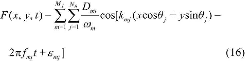
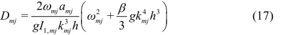
where Dmjcan be obtained from Eq.（9）， i.e.，

1.3.2 Fully reflective boundaries

For a fully reflective vertical boundary， the normal velocity must be zero. i.e.，

in whichn is the outward unit normal vector of the reflective boundary and nxand nyare the two components ofnalong the two spatial co-ordinates， respectively.

In fact， when the orientation of a boundary segment does not coincide with the global Cartesian axes，Eq.（18） is not easy to be treated in the finite element equation. To facilitate the treatment of the fully reflective boundary conditions at the points of the boundary that the orientation of the boundary segment does not coincide with the global Cartesian axes， a locally rotated coordinate system is introduced to rotate the Cartesian coordinate to the new coordinate system（n，T ）， in whichnis aligned with the outward normal andTis the tangent at the boundary node. The boundary condition can be resolved on the local coordinate system. Details can be found in Liu et al.［15］.

1.3.3 Absorbing boundaries

To eliminate the boundary reflections， a “sponge” layer is proposed to be placed in front of the absorbing boundaries to absorb the incoming wave energy. On the sponge layer， the surface elevation η andthe horizontal velocities（u，v）are divided by µ（x，y）at the end of each time step. The factor µ（x，y）takes the following form after extending the one-dimensional form to the two dimensional case.

in whichd is the distance between the point on the“sponge” layer and the boundary，∆dis the typical dimension of the elements，dsis the sponge layer width， usually equal to one or two wave lengths and δis a constant specified as 4 in this paper.

2. Verification of the numerical model

The numerical model was verified using typical examples［15］. To further show the effectiveness of the numerical model， a comparison of the numerical and physical results for the multidirectional wave diffraction through a breakwater gap is made in this paper. Figure 1 is the computational domain. The breakwater boundaries are taken as fully reflective boundaries instead of the absorbing boundaries used in the physical experiments by Yu et al.［18］. Because the reflected waves from the heads are the main part of the wave conditions in the harbor and an enough long breakwater head is used in the experime nts， the experimental data can be used to testify the calculated results. The thickness of the breakwater is 0.35 m. It is 4m away from the wave maker. The case of the breakwater gap width B=7.85min the physical model tests is selected in this paper. To use the source method described above， the waves are generated at the source linex= 0 m and the absorbing boundary is arranged at x= -4.0 m.

In the computation， the incident significant wave height Hs=0.05m， the peak period Tp=1.20s. The principal wave directionθ=0oand 45o. The dire-0ctional spreading parameters=19. The constant water depthh =0.4m. The time step ∆t=0.04s， the maximum side length of the element∆x=0.07m，and the total computation time is 163.8 s. The JONSWAP spectrum withγ=4is used. The numbers of frequencies and directional components are Mf=100and Nθ=36， respectively for the simulation of directional waves.

After the calculation， the computed wave diffraction coefficients in the harbor are calculated by

where Hi，1/3and HI，1/3are the diffraction significant wave height and the incident significant wave height， respectively.

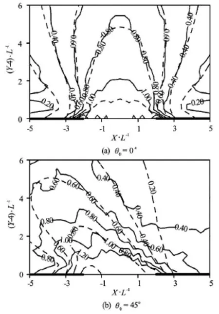
Fig.2 Comparison of the computed and experimental diffraction coefficients for multidirectional wave diffraction through breakwater gap （solid line: numerical results， dashed line: experimental results） （multidirectional waves: Hs=0.05m，Tp=1.20s，s =19）

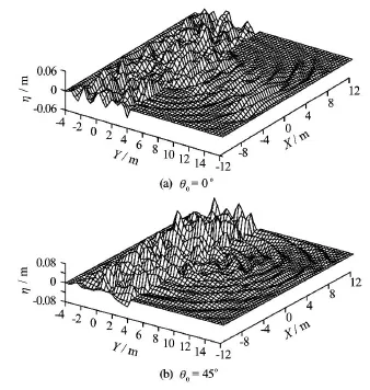
Fig.3 Perspective views of the multidirectional wave surface at t =160s（multidirectional waves:Hs=0.05m，Tp= 1.20 s，s =19）

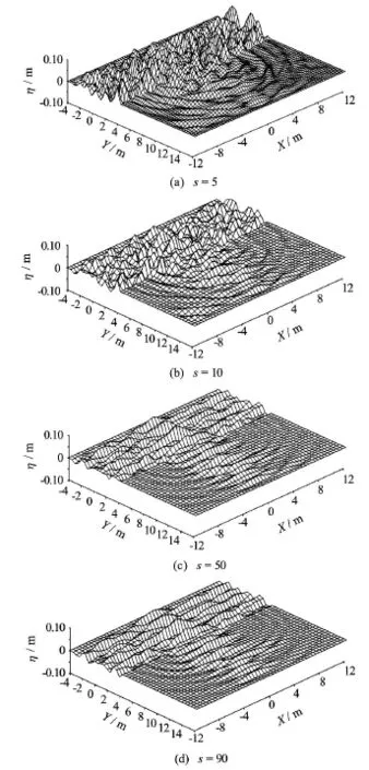
Fig.4 Perspective views of water surface for the wave diffraction through breakwater gap at instant time t=80s for different input directional waves

Figure 2 gives a comparison between the calculated diffraction coefficients and the experimental results， in whichL is the wave length corresponding to the peak period Tp. First， the distance between the wave generator and the breakwater is only 4m and the breakwater is a fully reflective boundary. Although the boundary conditions in front of the breakwaters used in the calculation are different from those in the experiments， the numerical results are very close to the experimental ones due to the same boundaries for the breakwater heads. That means that the source function method is very effective even if there are a great deal of reflected waves in the computation domain. Especially， the method is very effective for multidirectional waves. This is critical to the real application because real sea waves are multidirectional waves and their active absorption is a tough task for the numerical modeling due to the wave complexity. Figure 3 shows two examples of the water surfaceη at t= 160 s for the two cases. It can be seen from the figures that the water surface keeps a stable state after such a long time calculation despite a great deal of reflections from the breakwaters. However， the waves at the left side in front of the breakwater for θ=45ohave0a little larger amplitude than those forθ=0o. This is0reasonable because the side boundaries in front of the breakwater are also reflective boundaries.

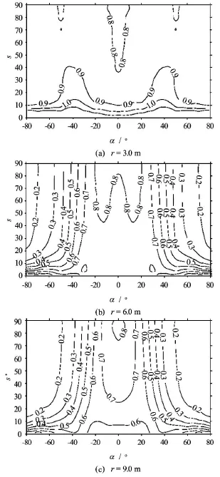
Fig.5 Distribution of the diffraction coefficients Kdwith the directional spreading parameters and along the transects α

Fig.6 Variations of the directional spectra in the harbor （r=8m）

3. Effects of wave directionality on the wave transformation

3.1 Effects of wave directionality on the wave diffraction through breakwater gap

To investigate the effects of the wave directional spreading on the wave diffraction through a breakwater gap， more calculations are carried out using the configuration shown in Fig.1. The wave parameters are Hs=0.05m，Tp=1.2s，Lp=1.93m，s=1-100（with ∆s=1）. The wave diffraction coefficients Kdat the three transects r =3 m， 6 m and 9 m， that is，r/Lp=1.55， 3.11 and 4.67 are calculated.

Figure 4 is the perspective views of the water surface for different directional spreading waves. It can be seen that the diffracted waves behind the breakwater with wide directional spreading （small value ofs） have larger amplitude than those with narrow directional spreading （large value ofs）. Toshow the quantitative effects of the wave directional spreading on the wave diffraction， Fig.5 gives the distribution of the diffraction coefficients Kdagainst the directional spreading parameters and along the transectsαfor r =3 m， 6 m and 9 m （r/Lp=1.55， 3.11 and 4.67）. It can be seen that the diffraction coefficients behind the breakwater （larger angleα） for small directional spreading parameters are larger than those for larges . The coefficient decreases with the increase ofs behind the breakwaters. However， the effects of the wave directional spreading on the diffraction coefficient can be neglected whens is larger than around 40 because the variation of the diffraction coefficients behind the breakwaters becomes very small. This conclusion is similar to that obtained from the wave diffraction around a semi-infinite breakwater by Li et al.［14］.

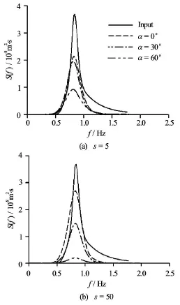
Fig.7 Variations of the frequency spectra in the harbor （r=8 m）

To show the variations of the directional spectra in the harbor due to the wave diffraction， the directional spectra at different positions in the harbor are analyzed using the Bayesian method. Figure 6 gives the input directional spectrum and the directional spectra at r =8m（r/L=4.15）and α=0o，30o，60oforpthe casess =5and s=50as examples. The variations of the directional spectra caused by the wave diffraction are recognizable. In different scales of vertical coordinates for differentα， it can be seen that the wave spectral density becomes smaller whenαis larger. Compared with the input directional spectrum，the shape of the spectrum sees a larger variation for smallers ， especially， the directional spreading becomes narrower. To show the tendency clearly， Fig.7 and Fig.8 give the variations of the frequency spectra and the directional spreading corresponding to the peak frequency due to the wave diffraction. Figure 7 shows that the shape of the frequency spectra is similar to each other， but a little wider than the input one. It is reasonable that the spectral density in the harbor is smaller than that of the input and the spectral density decreases with the increase of the angleα. For waves with input s =5， the spectra at r =8m，α= 0oand 30oare basically identical to each other because of the wider wave directional spreading. Also， it is evident that the spectral density behind the breakwater for narrow directional spreading waves is smaller than that for wide directional spreading waves. Figure 8 shows that the variation of the directional spreading at different points in the harbor is evident due to the wave diffraction. For the case of input waves with wide spreadings=5， the directional spreading function in the harbor becomes relatively narrower because of the wave diffraction. The main wave direction basically turns to be similar to the polar angle α. But for narrow waves in whichsis large， the variation of the directional spreading is not as large as that for wide directional waves.

Fig.8 Variation of the directional spreading in the harbor （r= 8 m）

Fig.9 Computation domain for wave transformation on a planar slope

Fig.10 Directional spectra at X =6mand X=16m

3.2 Effects of wave directionality on the wave transformation on a planar slope

To investigate the effects of the wave directionality on the wave transformation further， the multidirectional wave propagation over a 1:25 planar beach is simulated using the numerical model for different cases of multidirectional waves， in which the directional spreading varies from wider case to narrower case. Figure 9 is the computation domain. The incident waves are also generated by the source function method as discussed above. The width of the domain is 30 m. The water depth is constant as h=0.5mfor a distance of 7 m in front of the slope. To expand the effective area for multidirectional waves， the corner reflection method［14］is used. So the reflective boundaries on the two symmetrical side boundaries are used in the computation. At the right end of the domain， the water depth in a distance of 3 m keeps constant as h=0.1mand the absorbing boundary is used. The wave parameters areHs=0.05m，Tp=1.2s，s=2，5， 10， 30， 50 and 70 and the main wave direction θ=0o. The incident wave length corresponding to0the peak period is Lp=2.047m. The time step ∆t= 0.04 s， the maximum side length of the element ∆x= 0.05 m.

To show the variations of the directional spectra，Fig.10 gives the directional spectra at two points in the domain for waves with s=2 and 70 as examples. The high frequency harmonics， caused by the wave shoaling， can be observed from the figures. But the high frequency harmonics ofs=2are much smaller in amplitude than those ofs=70because of the effect of the wave directional spreading on the wave transformation. The figures show that for smallers， which means wider directional spreading， the directional spectrum at X =16m（h/Lp=0.068）becomes narrower in directional spreading because of the wave refraction. However， for the waves with inputteds= 70， the difference between the directional spectra at

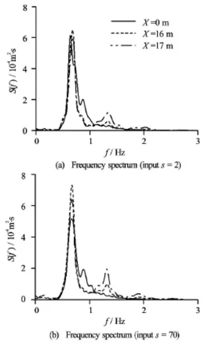
Fig.11 Variation of the frequency spectra over the slope

Fig.12 Variation of the energy of the generated higher harmonics at X =15 m， 16 m and 17 m （h/Lp=0.088， 0.068 and 0.049）

X =6m（h/Lp=0.244）and X =16m（h/Lp= 0.068）is not as large as that shown in Fig.10（a）. To show the spectral transformation further， Fig.11 gives the spectral variation for the waves with inputteds= 2 and 70. Comparing the two figures， the difference of the high frequency harmonics can be clearly observed. That means that the wave directional spreading has a definite effect on the generation of higher harmonics. For different directional spreading waves， the wave energy for higher harmonics Ei（i=1 and 2 represent the second and third harmonics） and the energy for the first wavesE0can be obtained from the integration of the analyzed frequency spectra. Figure 12 gives the variation of the relative energy Ei/E0at X=15 m，16 m and 17 m （h/Lp=0.088， 0.068 and 0.049） versus the directional spreading parameters. The figures show that the smaller the value of s， the less the energy of the generated higher harmonics. Similar to that shown above in the calculation of the wave diffraction，whensis larger than around 40， the effects of the wave directional spreading on the wave transformation can also be neglected.

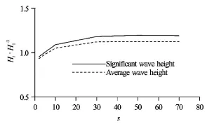
Fig.13 Relative wave height versus the directional spreading parameters（X =15m，h/Lp=0.088）

To investigate the effects of the wave directional spreading on the wave transformation further， the variation of the relative wave height at X =15m（h/ Lp=0.088）against the inputted directional spreading parametersis given in Fig.13. It is shown that the wave height at X =15m（h/Lp=0.088）increases with the increase ofs. However， similar to that shown in the wave diffraction to the harbour， the wave directional spreading has no evident effects on the wave height after the directional spreading parameter sis larger than around 40.

In addition， nonlinear effects in shallow water will distort the wave profile， creating higher， more peaked crests and flatter， broader troughs. The distortion and asymmetry of waves in shallow water is important for many coastal processes and can be measured by the skewness（λ3）and the kurtosis （λ4）of the water surface， i.e.，

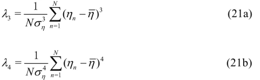
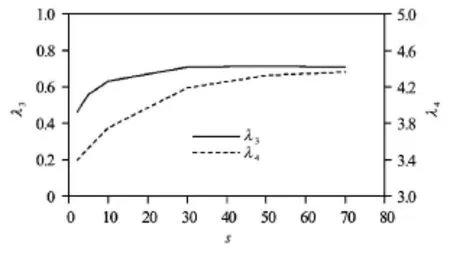
Fig.14 Variation of the skewness and kurtosis of the water surface at X =15m（h/Lp=0.088）versus directional spreading parameters

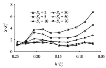
Fig.15 Variation of directional spreading parameter salong the center line

During the calculation， the directional spectra along the center line are analyzed and the directional spreading parameters can be obtained by fitting the analyzed results to Eq.（16）. The variations of the directional spreading parameters along the center line of the computational domain represented by the relative water depth is shown in Fig.15. In the figure，SImeans the inputted directional spreading parameters . The figure shows that the spreading parameter sgenerally becomes larger and larger along the slope in spite of the data scatter， which may be caused by the resolution of the analysis method for the directional spectrum. This is reasonable because of the wave refraction with different directional waves. However， again， when the inputted directional spreading parameters is larger than around 40， there is no evident difference for different spreading parameterss.

4. Conclusions

In this paper， a finite element model with an introduced source function method for solving the Boussinesq equations is proposed and applied to simulate the wave diffraction through a breakwater gap and the wave transformation along a planar bathymetry. The numerical model is effective for simulating the multidirectional wave transformation when a great deal of reflected waves exist in the computational domain.

The numerical results for the wave diffraction through a breakwater gap show that the wave directional spreading has a definite effect on the wave diffraction. The wave heights of wider multi-directional waves are larger in the sheltered areas behind the breakwater compared with those of narrower directional irregular waves. Wave directional spreading makes the wave heights behind the breakwater more uniform. However， in engineering sense， the effects of the wave directional spreading on the wave diffraction can be neglected when the directional spreading parameters is larger than around 40.

For the multi-directional wave transformation on a planar beach， the wave directional spreading restrains the generation of higher wave harmonics. For the same length of beach， the narrower the wave directional spreading， the larger the generated higher wave harmonics. The distortion and asymmetry of the waves become weaker for wider directional spreading waves. In addition， the directional spreading parameters becomes larger and larger during the wave transformation along the beach due to the wave refraction. However， the value of 40 fors can be used as a rough critical value for the evaluation of the effects of the wave directional spreading on the wave transformation. Whens is larger than around 40， the effects of the wave directional spreading on the wave transformation can be neglected.

References

［1］ FEDDERSEN F. Effect of wave directional spread on the radiation stress: Comparing theory and observations［J］. Coastal Engineering， 2004， 51（5-6）: 473-481.

［2］ ILLC S.， CHADWICK A. J. and FLEMING C. Detached breakwater: An experimental investigation and implication for design Part1 hydrodynamics［J］. Proceedings of the Institution of Civil Engineerings-Maritime Engineering， 2005， 158（3）: 91-102.

［3］ PUJIANIKI N.， KIOKA W. Nonlinear evolution of wave groups in directional sea［C］. Proceedings of 7th International Conference on Asian and Pacific Coasts. Bali， Indonesia， 2013.

［4］ NASERIZADEH R.， BINGHAM H. B. and NOORZADA. A coupled boundary element-finite difference solution of the elliptic modified mild slope equation［J］. Engineering Analysis with Boundary Elements， 2011，35（1）: 25-33.

［5］ HAMIDI M. E.， HASHEMI M. R. and TALEBBEYDOKHTI N. et al. Numerical modelling of the mild slope equation using localized differential quadrature method［J］. Ocean Engineering， 2012， 47: 88-103.

［6］ RUSU E.， GONCALVES M. and SOARES C. G. Evaluation of the wave transformation in an open bay with two spectral models［J］. Ocean engineering， 2011，38（16）: 1763-1781.

［7］ ILIC S， Van Der WESTHUYSEN A. J. and ROELVINK J. A. et al. Multidirectional wave transformation around detached breakwaters［J］. Coastal Engineering，2007， 54（10）: 775-789.

［8］ FUHRMAN D. R.， BINGHAM H. B. and MADSEN P. A. Nonlinear wave-structure interactions with a highorder Boussinesq model［J］. Coastal Engineering， 2005，52（8）: 655-672.

［9］ MADSEN P. A.， FUHRMAN D. R. High-order Boussinesq-type modeling of nonlinear wave phenomena in deep and shallow water. Advances in numerical simulation of nonlinear water waves［M］. Singapore: World Scientific， 2010， 245-285.

［10］ KAZOLEA M.， DELIS A. L. and NIKOLOS I. K. et al. An unstructured finite volume numerical scheme for extended 2D Boussineq-type equations［J］. Coastal Engineering， 2012， 69: 42-66.

［11］ STEINMOELLER D. T.， STASTNA M. and LAMB K. G. Fourier pseudospectral methods for 2D Boussinesqtype equation［J］. Ocean Modelling， 2012， 52-53: 76-89.

［12］ FANG Ke-zhao， ZHANG Zhe and ZOU Zhi-li et al. Modelling of 2-D extended Boussinesq equations using a hybrid numerical scheme［J］. Journal of Hydrodynamics， 2014， 26（2）: 187-198.

［13］ DARIPA P. Higher order Boussinesq equation for two way propagation of shallow water waves［J］. European Journal of Mechanics B/Fluids， 2006， 25（6）: 1008-1021.

［14］ LI Y.， LIU S. and YU Y. et al. Numerical modelling of multi-directional irregular waves through breakwaters［J］. Applied Mathematical Modelling， 2000， 24（8-9）: 551-574.

［15］ LIU S.， SUN Z. and LI J. An unstructured FEM model based on Boussinesq equations and its application to the calculation of multidirectional wave run-up in a cylinder group［J］. Applied Mathematical Modelling， 2012，36（9）: 4146-4164.

［16］ SUN Zhong-bin， LIU Shu-xue and LI Jin-xuan， Numerical study of multidirectional focusing wave runup on a vertical surface-piercing cylinder［J］. Journal of Hydrodynamics， 2012， 24（1）: 86-96.

［17］ BEJI S.， NADAOKA K. A formal derivation and numerical modelling of the improved Boussinesq equations for varying depth［J］. Ocean Engineering， 1996， 23（8）: 691-704.

［18］ YU Y.， LIU S. and LI Y. et al. Refraction and diffraction of random waves through breakwater［J］. Ocean Engineering， 2000， 27（5）: 489-509.

10.1016/S1001-6058（15）60533-9

（February 21， 2014， Revised May 12， 2014）

* Project supported by the National Natural Science Foundation of China （Grant Nos. 51079023， 51221961 and 51309050）， the National Basic Research Development Program of China （973 Program， Grant Nos. 2013CB036101，2011CB013703）.

Biography: LIU Shu-xue （1965-）， Male， Ph. D.， Professor

LI Jin-xuan， E-mail: lijx@dlut.edu.cn