
具有加强诊断措施的Filippov HIV/AIDS 传染病模型
2020-11-04 03:06王爱丽
工程数学学报 2020年5期
王爱丽
(宝鸡文理学院数学与信息科学学院,宝鸡 721013)
1 Introduction
Over the recent few decades, human immunodeficiency virus (HIV), which causing acquired immune deficiency syndrome (AIDS), has advanced to a chronic condition needing early and lifelong treatment, although it is an infection invariably culminating in AIDS. Almost all the world try to curb this epidemic and mitigate its impact.However, there are still a lot of problems and many challenges although the endeavors can help to prevent the replication of virus and to maintain the normal CD4+T cell counts[1]. Therefore, evaluating the effectiveness of variable control measures becomes important for the public health sector to control HIV[2]. Besides the highly active antiretroviral therapy(HAART),HIV counselling and testing(HCT)play an important role in HIV prevention[3-6].
Although the proportion of the diagnosed HIV individuals is increasing,many HIVinfected people have not yet been diagnosed. Johnson et al. shows that the undiagnosed HIV-positive individuals contribute to a disproportionate and large fraction of HIV transmission[3]. They also suggest that a frequency of HIV testing likely has a strong impact on the effect of antiretroviral treatment. It is a considerable number of those living with HIV but unaware of their infection. In European countries, the proportion of infected individuals who are undiagnosed is greater than 20%[5,6]. It is found that those individuals unaware of their HIV infection are 3.5 times more likely to transmit the virus than those aware of being infected[7]. Increasing the rates of HIV testing is certainly vital and can aid to plan interventions, but a number of practical challenges occur in monitoring the rate of HIV diagnosis in HIV-positive individuals[3]. So it is necessary to explore how to implement the diagnosis measure quantitatively and qualitatively. And mathematical modeling is a good choice.
In fact,mathematical modeling,as an effective method,has been adopted by many scientists to identify the infection factors in HIV controlling[2,8-15]. Based on the clinical progression of disease and epidemiological status of the individuals, an epidemic model is proposed to study the epidemic trend and the future in China[2]. The diagnosis rate is assumed to be a constant in this model. In HIV control practice, how to implement the diagnoses measure varies as the total number of HIV-diagnosed cases varies. An enhanced diagnosis rate should be taken once the number of HIV-diagnosed individuals is above a certain level. If we quantifying this issue by a mathematical model, it will result in a Filippov model[16]. Filippov system has been adopted by some scientists to study the epidemic disease control[17-21]. In [20,21], we have investigated the impact of the switching control measure on the general epidemic disease. In [17-19], the authors have formulated Filippov models to study the control outcome of the infected HIV virus within hosts. However, few work has been found on the HIV control by formulating Filippov model between hosts. And it falls within the scope of this work.
The aim of this work is to explore how the repeatedly enhanced diagnosis strategy affects the HIV transmission. The rest of this paper is as follows. In the next section,we will formulate the Filippov model and present some preliminaries. In the third section, we will examine the dynamics of the subsystems as well as the sliding mode dynamics. The global behavior of the Filippov system is investigated in the fourth section. And the conclusion and the biological remarks are given in the last section.
2 Filippov HIV epidemic model
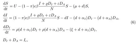
As suggested in the introduction, an enhanced diagnosis measure is initiated repeatedly when the number of diagnosed cases exceeds a certain level. To illustrate our idea, we will construct a simple Filippov system to model the diagnosis measure: once the number of the diagnosed cases (defined by DI+DA) exceeds the critical level, the enhanced diagnose measure is triggered; otherwise, the general diagnosis measure is carried out. We only focus on the high-risk population and assume all AIDS cases have been diagnosed[12,13]. We classify the high-risk population group into four subgroups:high-risk susceptibles S, HIV infected but not yet diagnosed I, diagnosed HIV-positive individuals who have not yet progressed to AIDS DI,and those with clinical AIDS DA.The model equations take the form
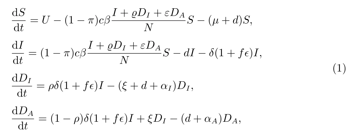
with
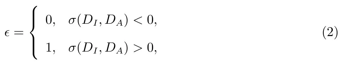
where σ(DI,DA)=(DI+DA)-Ic. In this model, N =S+I+DI+DAdenotes the size of the high-risk population, who become infected at a rate
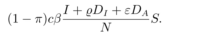
The parameter β denotes the probability of transmission per high-risk behavior (i.e.sexual action or needle sharing); c represents the contact rate, i.e., the rate of acquisition of needle-sharing partners or new sexual; π is the degree of intervention due to methadone treatment or condom use; ϱ and ε are the relative infectiousness of the diagnosed HIV-positive individuals and AIDS patients; δ stands for the diagnosis rate;ρ is the proportion of diagnosed individuals who are HIV positive; ξ is the rate of progression from HIV diagnosis to AIDS class; αIand αAdenote additional death rates for the diagnosed HIV-positive individuals and for those living with AIDS,respectively.Although individuals with HIV do not die directly from the disease,suicide rate is high among HIV-positive individuals in China[22]. The initial data and parameter values are summarized in Table 1.

Table 1 Initial data and parameters used in the model
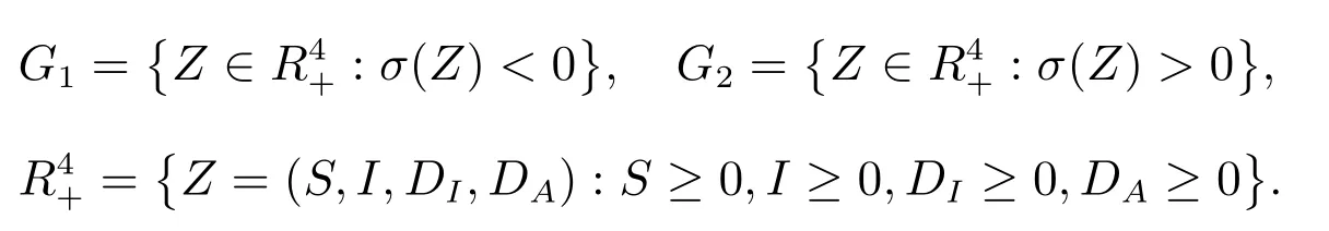
Denote Z =(S,I,DI,DA) and
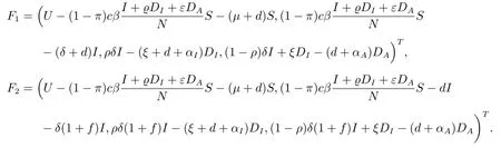
System (1) with (2) can be written as the following Filippov system[16]
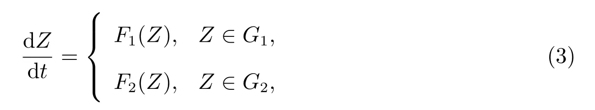
where

In the following,we introduce two types of singular points which play an important role in the rest of this paper.


Both the real equilibria and virtual equilibria are called regular equilibria.
Definition 2If there is a point Z*satisfying σ(Z*)=0 and
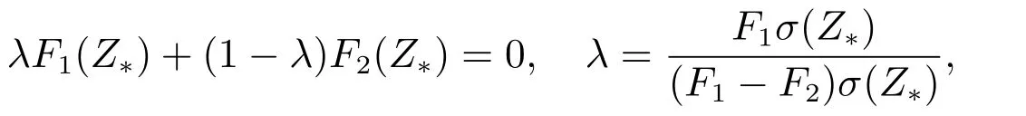
then Z*is called a pseudo-equilibrium of system(3),where Fiσ(Z)=Fi(Z)· grad σ(Z)is the Lie derivative of σ with respect to the vector field Fiat the point Z.
3 Dynamics of subsystems
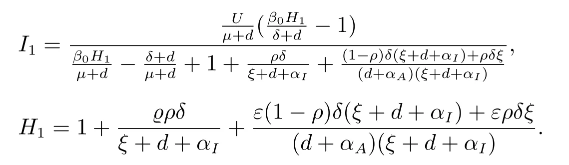
Subsystem S1possesses a disease-free equilibrium E0= (U/(μ+d),0,0,0). By using the next-generation matrix method[23],we can get the basic reproduction number for subsystem S1as follows


Further discussion yields the following result.
Theorem 1If R01<1, the DFE E0is locally asymptotically stable; if R01>1,the DFE E0is unstable.
ProofEvaluating the Jacobian matrix of subsystem S1at the DFE, we get a negative characteristic root -μ-d with others satisfying

where
A1=3d+αA+ξ+αI+δ-β0,
A2=-β0εδ(1-ρ)+(ξ+d+αI)(δ+d-β0)-β0ϱρδ+(d+αA)(ξ+2d+αI+δ-β0),
A3=-β0εδξ-β0ε(1-ρ)δ(d+αI)+(d+αA)[(ξ+d+αI)(δ+d-β0)-β0ρϱδ].
One can easily get that

It follows that
Note that
A1A2-A3>(d+δ)(ξ+d+αI)εδ[ξ+(d+αI)(1-ρ)]+(d+αA)2(ξ+d+αI)2+(d+αA)εδ(1-ρ)(ξ+d+αI)2+(d+αA)2(ξ+d+αI+d+δ)ϱρδ >0,
so all the roots of (4) are negative, according to the Hurwitz criteria. Hence, the DFE E0is locally asymptotically stable for R01<1. If R01>1, we can get A3<0, so the DFE E0is unstable. This completes the proof.
For subsystem S2, by implementing the similar discussion, we can get that the disease-free equilibrium E0is locally asymptotically stable when R02<1, where

Note that the dynamics in each subregion Gi(i = 1,2) is defined well; while the dynamical behavior of system (3) on the discontinuous boundary Σ is not clear up to this point. So in the following, we focus on the dynamics of system (3) on Σ, i.e., the sliding mode dynamics. To this end, we initially examine the nature of the discontinuous surface Σ. In fact, there are three possible subregions according to whether the trajectories for the two subsystems moving toward Σ or away from Σ. Denote Zc=(S,Ic,DI,DA) and we distinguish the following three regions
sliding region Σs={Zc∈Σ:〈σZ(Zc),F1(Zc)〉≥0,〈σZ(Zc),F2(Zc)〉≤0};
crossing region Σc={Zc∈Σ:〈σZ(Zc),F1(Zc)〉〈σZ(Zc),F2(Zc)〉>0};
escaping region Σe={Zc∈Σ:〈σZ(Zc),F1(Zc)〉≤0,〈σZ(Zc),F2(Zc)〉≥0}.
Direct calculation gives no escaping region; while the sliding mode region takes the following form

with


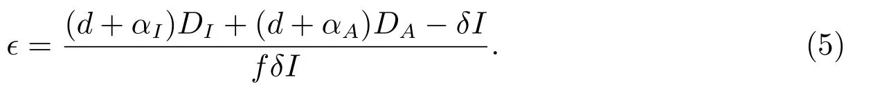
Substituting (5) into equation (1) gives the sliding mode dynamics as follows

If we further have , Esis a pseudo-equilibrium of the Filippov system (3).
4 Results


Figure 1 A simulation of typical solutions of the Filippov system (3)for Case 1 with Ic =1.0398×10⁷, f =0.3
According to the above discussion, the threshold value and the enhanced diagnosis rate play important roles in determining the duration of ordinary diagnosis measure and that of the enhanced diagnosis rate. So in the next,we explore how the threshold value Icaffects the duration. We choose the threshold value Icas a bifurcation parameter and let it vary from DI2+DA2to DI1+DA1with other parameters and initial values fixed as those in Table 1. We record the switch numbers as well as the durations of the ordinary diagnosis measure and that of the enhanced diagnosis measure, as shown in Figure 2.

Figure 2 The impact of the threshold value Ic on the duration of the ordinary diagnose measure and the enhanced diagnose measure and switches of the two types of measures
It follows from Figure 2 that the duration of the ordinary diagnosis measure increases as the increasing of the threshold level Ic; while the duration of the enhanced diagnosis measure decreases as Icincreases. For every specified value of Ic,the duration of the ordinary diagnosis measure will stabilize at a certain level. So does the duration of the enhanced diagnosis measure. This suggests that how often the diagnosis measures switch from the ordinary one to the enhanced one or the reversed is determined if the threshold level and other parameters are specified. This allows us to make a regime about diagnosis. With this duration regime, we can implement the switching diagnosis measures without evaluating whether the diagnosed cases exceeds the threshold level.This is helpful in designing the diagnosis plan in practice.
We further know that the second duration of the ordinary diagnosis measure dramatically decreases compared to the first duration, as shown in Figure 2(a). And it gradually approaches a steady level since then. It is also true for the enhanced diagnosis measure, as shown in Figure 2(b). Comparing Figure 2(a) with Figure 2(b) gives that the duration of the enhanced diagnosis measure is more sensitive than that of the general diagnosis measure to the the threshold value Ic. So it is necessary to choose the duration of ordinary/enhanced diagnosis measure carefully.
To investigate the control outcome of the switching diagnosis measure mathematically, the phase plane plot of the number of the HIV infected not diagnosed cases, the number of the diagnosed HIV-positive cases not progressed to AIDS and the number of the clinical AIDS cases are given in Figure 3. A pseudo-equilibrium Esexists for the Filippov system (3) in this case, as shown in Figure 3. The shaded region in Figure 3 represents the sliding mode region Σswhile the crossing region Σcis unshaded.Projection of five solutions of Filippov system (3) in the subspace DI-DA-I with different initial values are plotted to show the stability of the crossing cycle. Points E1,E2and Esrepresent the projection of the equilibrium of the free system S1, the equilibrium of the control system S2and the pseudo-equilibrium of Filippov system(3), respectively. Figure 3 shows that the two regular equilibria Ev1and Ev2as well as the pseudo-equilibrium Esare not stable. And there exists a crossing cycle, which acts as the global attractor of the Filippov system (3) in this case. All the five trajectories ultimately tend to the crossing cycle. Some of the trajectories slide on the sliding mode region Σsfirstly, then cross the discontinuous boundary Σc, and finally approach the crossing cycle. Some of them cross the crossing region firstly and then go to the crossing cycle. This implies the global stability of the crossing cycle. Biologically, whatever the initial condition is,the number of the HIV infected not diagnosed cases(I),the number of the diagnosed HIV-positive cases not progressed to AIDS (DI) and the number of the clinical AIDS cases (DA) can be contained below a certain level while they always fluctuate.


Figure 4 A simulation of typical solutions of Filippov system (3)for Case 2 with f =0.3, Ic =9.5×10⁶

If we increase the threshold value Icsuch that Ic>DI1+DA1, the endemic equilibrium E2of the control system is virtual while the endemic equilibrium E1of the free system is real. And no pseudo-equilibrium exists for the Filippov system (3), as shown in Figure 5.

Figure 5 A simulation of typical solutions of Filippov system (3)for Case 3 with f =0.3, Ic =1.2×10⁷

5 Conclusion and biological discussion
We have formulated a Filippov model to describe the impact of the enhanced diagnosis policy on HIV control. The diagnosis strategy is defined as follows: once the number of the diagnosed HIV individuals is above a certain level, the enhanced diagnosis measure is initiated; otherwise, only a general diagnosis measure is adopted.It is indeed a non-smooth model, which is distinct to the smooth counterpart. This modeling allows us to explore how the switching diagnosis policy affect the process of HIV transmission as well as the control outcome.

Compared to those models with constant diagnosis ratio, we have formulated a simple Filippov model to investigate how the enhanced diagnosis measure affect HIV control in this paper. The number of the HIV infected cases can fluctuate around the priori level if we choose an appropriate threshold value. This is new compared to the conclusion for those model with constant diagnosis ratio. This threshold policy helps to provide a new insight into HIV control.
猜你喜欢
山西大同大学学报(自然科学版)(2022年1期)2022-03-17
科技进步与对策(2020年19期)2020-10-15
大众文艺(2020年15期)2020-09-11
中学数学研究(江西)(2020年7期)2020-07-22
大众文艺(2019年23期)2019-12-15
唐都学刊(2018年3期)2018-06-12
当代陕西(2018年6期)2018-05-22
当代陕西(2017年12期)2018-01-19
音乐天地(音乐创作版)(2017年1期)2017-04-24
中国卫生(2016年11期)2016-11-12
