
椭圆特征值问题的局部径向基函数差分法
2020-11-04 03:07冯新龙
工程数学学报 2020年5期
张 毅, 冯新龙
(新疆大学数学与系统科学学院,乌鲁木齐 830046)
1 Introduction
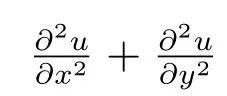
In this paper, we investigate the two dimensional elliptic eigenvalue problem followed by
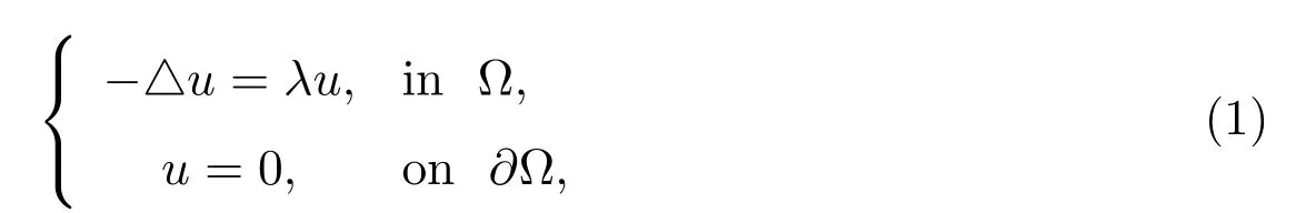
where the region Ω ⊆R2, λ is the eigenvalue and u represents the eigenvector. The problem is to find an eigenpair (λ,u) for which λ >0 and u is non-null satisfying (1).
Numerical methods for eigenvalue problems have become attractive in the field of fluid mechanics. In the past, various approaches had been proposed to solve these problems. Xu and Zhou[1]proposed a two-grid discretization for eigenvalue problems.Two kinds of two-grid new mixed finite element schemes for the elliptic eigenvalue problem based on less regularity of flux are considered in [2]. These methods are wellestablished,but all suffer certain drawbacks due to their reliance on a mesh of elements connected in a predefined way. Because of these limitations, various meshless methods had been proposed for solving PDEs in engineering applications.
As one kind of meshless method, radial basis functions (RBFs) have been increasingly popular in approximation theory. The discovery of the RBF interpolation method itself is attributed to Hardy in 1971, who used the Multiquadric (MQ) RBF for scattered data interpolation in 2D to solve problems in topography[3]. In 1990, the application of RBFs as a mesh-free method for partial differential equations (PDEs)was first proposed by Kansa[4,5]. RBF-based methods are attractive because they are simple to apply and geometrically flexible, capable of handling complicated domains on scattered nodes with no need for a computational mesh. But its main drawback is ill-conditioning of the resulting linear system as the number of nodes is increased[6]. To overcome the drawback of the global RBF method, a local RBF method has recently been put forward independently by several authors[7-10]. The method uses RBFs with global support,but the approximation is carried out at a given node with some nearest neighbors instead of all nodes in the global region. The local RBF method can also be considered as a generalization of the classical finite difference(FD)method to scattered node layouts, we refer to the local RBF method as the RBF-generated finite difference(RBF-FD) method, as in[8].
In this paper,the local RBF-FD method is extended for solving the elliptic eigenvalue problem. We present the numerical results for three kinds of RBFs using structured and unstructured node layouts to testify the accuracy of the method compared with the analytical solutions. We also study the effect of the shape parameter in the formulas of the RBF-FD method for elliptic eigenvalue equation on the unit square numerically.
The rest of the paper is structured as follows. In section 2, a brief introduction to radial basis functions is presented. The main results of this study are contained in section 3,where we establish the formulation of the RBF-FD scheme and apply the local RBF-FD approximations for the elliptic eigenvalue problem. In section 4, numerical experiments are given, showing that our proposed approaches are very efficient for several node layouts on different domains. And conclusions are drawn in section 5.
2 Radial basis functions

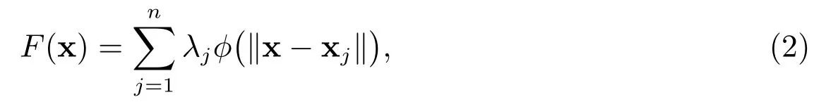
where φ(r), r =‖x-xj‖≥0,is some radial function,the norm‖x-xj‖is usually the Euclidean distance between nodes x and xj, and n is the total number of nodes. The unknown expansion coefficients λj, j = 1,2,··· ,n are determined by F(xi) = fi, i =1,2,··· ,n, which leads to the following symmetric linear system
There are two types of traditional RBFs: piecewise smooth RBFs and infinitely smooth RBFs. If φ is one of the piecewise smooth RBFs without shape parameters,we will obtain the RBF interpolation explicitly after solving the linear system. On the other hand, if φ is one of the infinitely smooth RBFs with a positive constant c which is known as the shape parameter, then suitable choices of the shape parameters are required to make[11]. In this paper,we choose the infinitely smooth RBFs for numerical approximation and discuss the effect of shape parameter c in section 3. Some commonly used RBFs are shown in Table 1.

Table 1 Some commonly used radial functions φ(r)
3 Meshless method formulation
3.1 RBF-FD weights
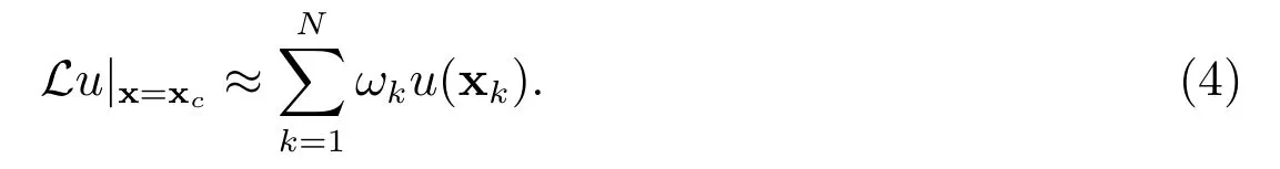
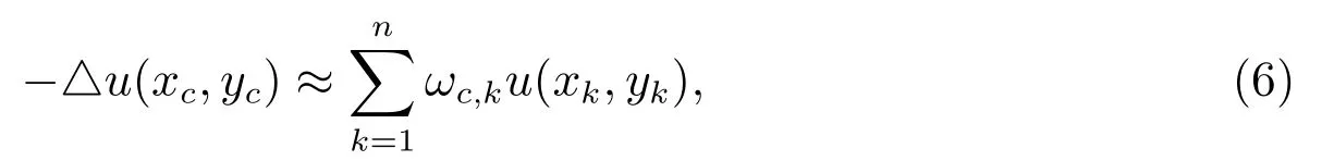
In this section, we describe how the RBF-FD formulas are derived and how the weights are exactly calculated. We consider an influence domain (or stencil) consisting of N scattered nodes x1,x2,··· ,xNand a differential operator L. For a given node xc,we want to approximate Lu(xc) by a linear combination of the function values of u at the N nodes, that is
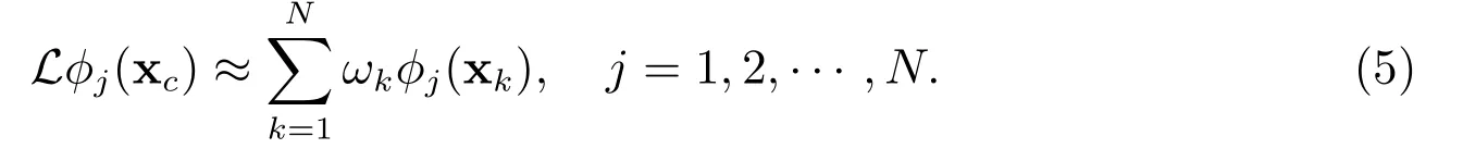
To determine the value of ωk,we choose a set of RBFs φi(x), i=1,2,··· ,N. This leads to the following linear system
3.2 Local RBF-FD formulas for the elliptic eigenvalue problem
the combined RBF and polynomial interpolant is assumed to be a linear combination of the radial and polynomial functions, thus it takes the form

with the constraints


Although (7) is well-posed without any augmented polynomials for the MQ, GA,and IMQ RBFs in Table 1, we augmented the radial functions with a constant β in this study, in order to maintain the condition that the RBF-FD formulas are exact for constants[13]. Substituting (7) into (6) and imposing the condition (9) leads to the symmetric, linear system of equations
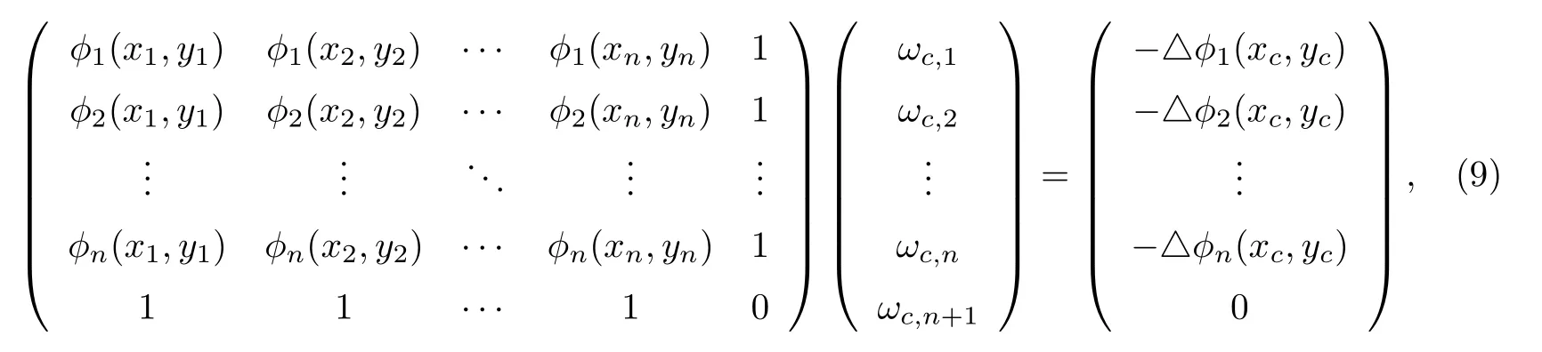
The discretization of (1) leads to an algebraic eigenvalue problem

The N ×N matrix L is the DM which is constructed by the RBF-FD weights calculated at each node and u=(u1,u2,··· ,uN)T. The element Li,jof this matrix can be expressed as follows
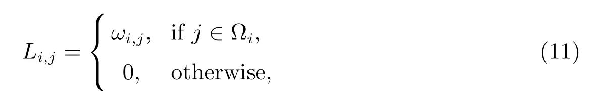
where Ωirepresents the set of neighbor nodes for node (xi,yi) in the influence domain.With the matrix assembled, the inverse power method is required to solve the problem for the first eigenvalue λ1,hwhich will be compared to the analytical solution to determine the accuracy of the local RBF-FD method. Now, the corresponding discrete problem is to find eigenpairs (λ1,h,u1,h) for which u1,his non-null and ‖u1,h‖0=1.
3.3 Choice of the local influence domain
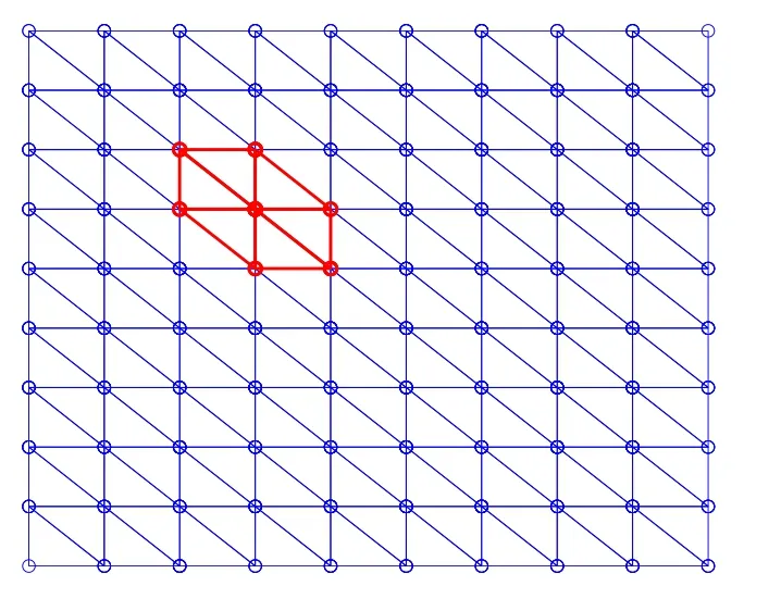
Figure 1 Choice of neighbors by links
4 Numerical results
In this section, the numerical experiments are carried out using Matlab. For the sake of simplicity,we just consider the first eigenvalue of the elliptic eigenvalue problem,applying Gaussian elimination and the inverse power method to solve the system(9)and find the first eigenvalue of (10), respectively. The relative error between an analytical and a numerical result is defined to be

where λ1,adenotes the first eigenvalue analytically and the numerical result is λ1,h.Noted that the total error in this work includes the error from the RBF-FD approximation, the linear system solver, and the inverse power method for the eigenvalue problem (10).
4.1 Unit square
The first example is to consider the elliptic eigenvalue model problem (1) on the unit square Ω=(0,1)×(0,1), the eigenvalues and eigenvectors are
λk,l=π2(l2+k2), l,k =1,2,··· ,∞,
and
uk,l(x,y)=sin(kπx)sin(lπy).
In Figure 2, we show three different node layouts in Ω: uniformly distributed nodes, nodes distributed randomly, and uniformly distributed nodes perturbed randomly within a radius of 0.3h from their original position, where h is the distance between adjacent uniform nodes.
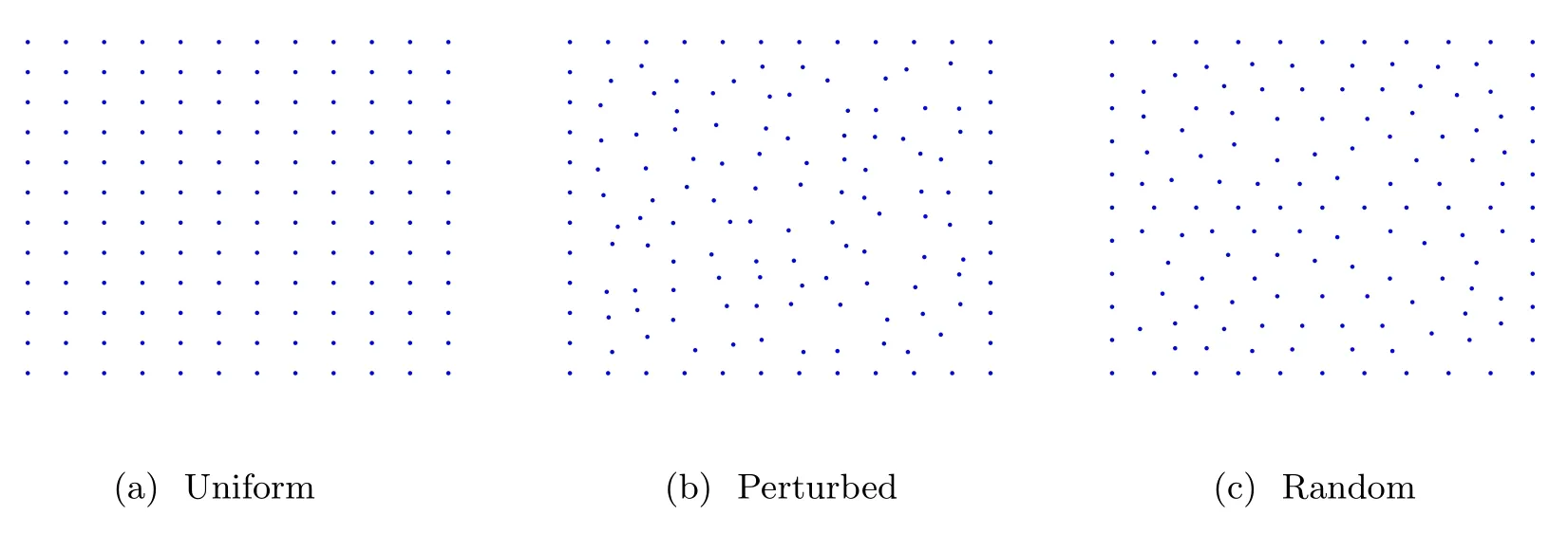
Figure 2 Three different layouts of the original points: uniform nodes,Perturbed nodes and Random nodes
Figure 3 shows the relative error ϵras a function of the total number of nodes N.We use the multiquadric RBFs with shape parameter c=1, and results are shown for three different node layouts in Figure 2. It can be seen from the figure that the relative error ϵrdecreases with the increasing of the number of nodes in all of the three layouts,and all the three cases give accurate results when there is enough points. And from the figure we can get that the best accuracies come from the uniform layout of point.
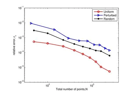
Figure 3 Relative error ϵr as a function of the total number of nodes N for three node layouts using MQ RBF-FD method with c=1
The convergence rates for the local RBF-FD method are presented according to Figure 4, where we show the relative errors of the method, using uniformly distributed nodes, as a function of the distance h between adjacent uniform nodes. Applying the least square fitting the data, we find convergent rate of GA RBF O(h2.2), MQ RBF O(h2.5),and IMQ RBF O(h2)which shown that MQ RBF interpolation is more efficient.
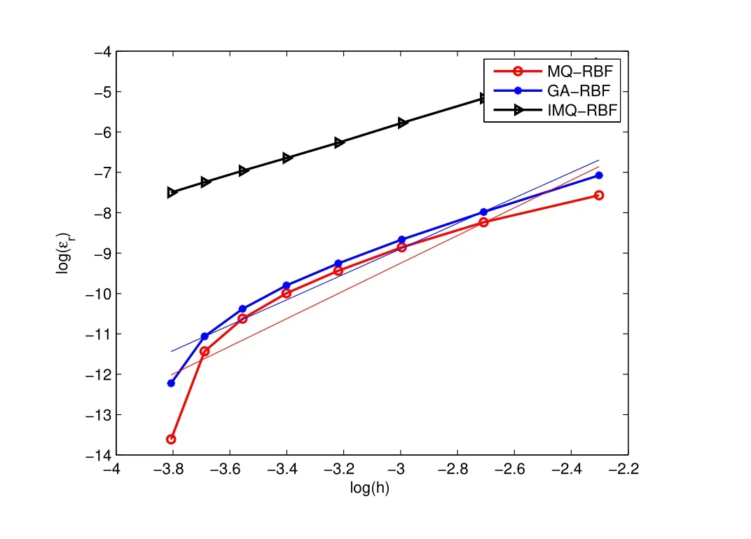
Figure 4 Plot shows log(ϵr) against log(h) for the MQ RBF-FD method with c=1 in the uniformly distributed nodes, to determine the orders of convergence
Figure 5 shows the results of finding the optimal shape parameter c with a fixed number of nodes N = 2500 for this method, using uniformly distributed nodes, uniformly distributed nodes perturbed randomly, and nodes distributed randomly. It can be seen that there exists an optimal value of the shape parameter that minimizes the error in all layouts and the results become more accurate as the shape parameter increases toward 1, but oscillatory nature for large values of c. We can also get that the optimal value is independent of the nodal distance and only depends on the value of the function, matching the result in [15,16].
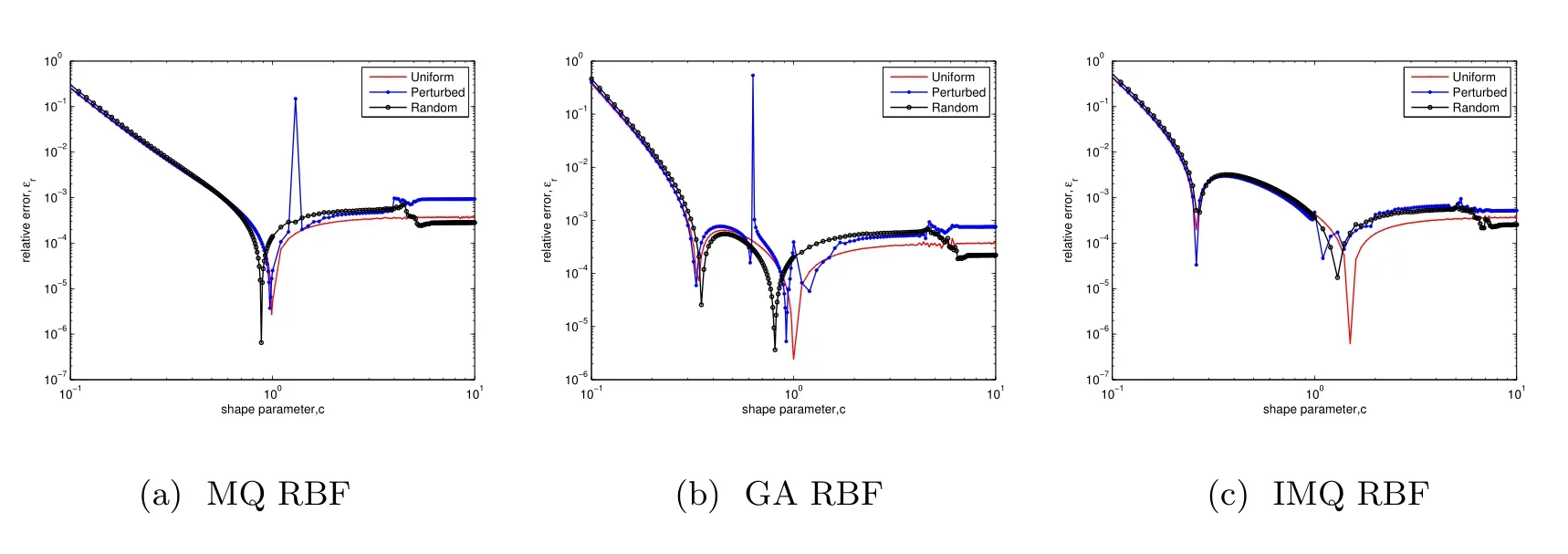
Figure 5 Relative error ϵr as a function of shape parameter c in RBF-FD method using 2500 points
Further, we presented the performance of the local RBF-FD method using various different RBFs(MQ,GA and IMQ)in Figure 6. We show relative error ϵras a function of the total number of nodes N, operating in three different layouts with c=1. All the point layouts show that errors in MQ RBF and GA RBF are better than in IMQ RBF.

Figure 6 Relative error ϵr as a function of the total number of nodes N for uniformly distributed, perturbed, and random nodes using the MQ, GA and IMQ RBFs with c=1 in the local RBF-FD method
Moreover, we give the plots of eigenvector u1,hof the first eigenvalue λ1,hat N =2500 nodes using MQ RBF-FD method with c=1 in Figure 7.

Figure 7 Plot of the eigenvector u1,h of the first eigenvalue λ1,h at N =2500 nodes:using MQ RBF-FD method with c=1 for the three node layouts
4.1 L-shaped domain
The second example is the elliptic eigenvalue model problem (1) on the L-shaped domain Ω=(-1,1)2[0,1]2. A reference value for the first eigenvalue of(1)is 9.639724 from[17]. Figure 8 illustrates the convergence of GA, MQ and IMQ RBF in three different point layouts. The results from the experiment show that each aspect is similar to the first example which is computed on the unit square, only slightly lower in accuracy.
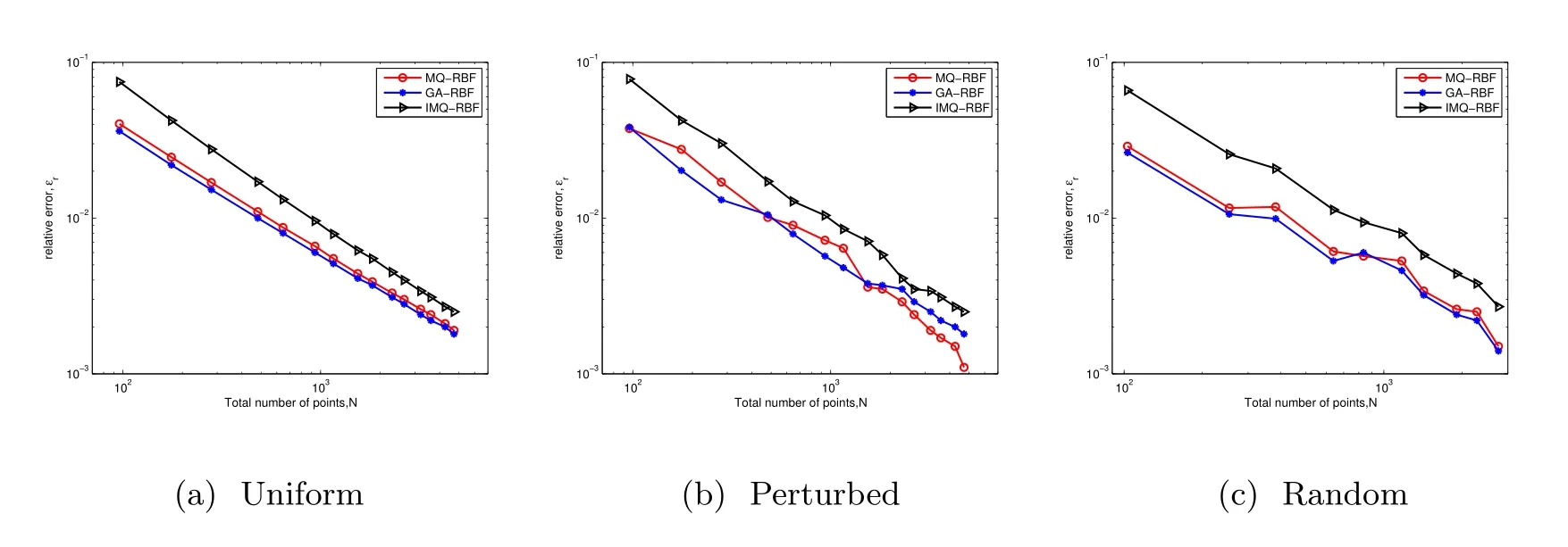
Figure 8 Convergence of GA, MQ and IMQ RBF in three nodal distribution
5 Conclusion
An elliptic eigenvalue problem is solved in this paper using the local RBF-FD method on the unit square region and L-shaped domain. The numerical results using regular and irregular node layouts show the excellent agreement with the analytical solutions. In comparison, we can find that the results obtained using uniformly distributed nodes is better than those obtained from perturbed and random points. In addition, it is found that MQ RBF and GA RBF display better results for the Laplace eigenvalue problem. But the IMQ RBF-FD is the most stable one. For each RBF-FD formula there is an optimal value of the shape parameter c for which the error is minimum. This value is independent of h and only depends on the value of the function and its derivatives at the nodes. In the future, we will extend the local RBF-FD method to more complex problems.
猜你喜欢
科技进步与对策(2022年19期)2022-10-08
湖南理工学院学报(自然科学版)(2022年1期)2022-03-16
空间科学学报(2020年6期)2020-07-21
校园英语·月末(2020年2期)2020-05-19
智富时代(2018年12期)2018-01-12
智富时代(2018年12期)2018-01-12
新疆农垦科技(2016年10期)2016-06-15
新疆大学学报(哲学社会科学版)(2015年1期)2015-10-13
新疆大学学报(哲学社会科学版)(2015年4期)2015-10-12
振动工程学报(2014年2期)2014-03-01
