Efficient and High-quality Recommendations via Momentum-incorporated Parallel Stochastic Gradient Descent-Based Learning

Xin Luo, Senior Member, IEEE, Wen Qin, Ani Dong, Khaled Sedraoui, and MengChu Zhou, Fellow, IEEE

Abstract—A recommender system (RS) relying on latent factor analysis usually adopts stochastic gradient descent (SGD) as its learning algorithm. However, owing to its serial mechanism, an SGD algorithm suffers from low efficiency and scalability when handling large-scale industrial problems. Aiming at addressing this issue, this study proposes a momentum-incorporated parallel stochastic gradient descent (MPSGD) algorithm, whose main idea is two-fold: a) implementing parallelization via a novel datasplitting strategy, and b) accelerating convergence rate by integrating momentum effects into its training process. With it, an MPSGD-based latent factor (MLF) model is achieved, which is capable of performing efficient and high-quality recommendations. Experimental results on four high-dimensional and sparse matrices generated by industrial RS indicate that owing to an MPSGD algorithm, an MLF model outperforms the existing state-of-the-art ones in both computational efficiency and scalability.

I. INTRODUCTION

BIG date-related industrial applications like a recommender systems (RS) [1]–[5] have a major influence on our daily life. An RS commonly relies on a high-dimensional and sparse (HiDS) matrix that quantifies incomplete relationships among its users and items [6]–[11]. Despite its extreme sparsity and high-dimensionality, an HiDS matrix contains rich knowledge regarding various patterns [6]–[11] that are vital for accurate recommendations. A latent factor (LF)model has proven to be highly efficient in extracting such knowledge from an HiDS matrix [6]–[11].

In general, an LF model works as follows:

1) Mapping the involved users and items into the same LF space;

2) Training desired LF according to the known data of a target HiDS matrix only; and

3) Estimating the target matrix’s unknown data based on the updated LF for generating high-quality recommendations.

Note that the achieved LF can precisely represent each user and item’s characteristics hidden in an HiDS matrix’s observed data [6]–[8]. Hence, an LF model is highly efficient in predicting unobserved user-item preferences in an RS.Moreover, it achieves fine balance among computational efficiency, storage cost and representative learning ability on an HiDS matrix [10]–[16]. Therefore, it is also widely adopted in other HiDS data related areas like network representation[17], Web-service QoS analysis [3], [4], [18], user track analysis [19], and bio-network analysis [12].

Owing to its efficiency in addressing HiDS data [1]–[12], an LF model attracts the attention of researchers. A pyramid of sophisticated LF models are proposed, including a biased regularized incremental simultaneous model [20], singular value decomposition plus-plus model [21], probabilistic model [13], non-negative LF model [6], [22]–[27], and Graph regularized Lpsmooth non-negative matrix factorization model [28]. When constructing an LF model, a stochastic gradient descent (SGD) algorithm is often adopted as a learning algorithm, owing to its great efficiency in building a learning model via serial but fast-converging training [14],[20], [21]. Nevertheless, as an RS grows, its corresponding HiDS matrix explodes. For instance, Taobao contains billions of users and items. Although the data density of a corresponding HiDS matrix can be extremely low due to its extremely high dimension, it has a huge amount of known data. When factorizing it [21]–[28], a standard SGD algorithm suffers from the following defects:

1) It serially traverses its known data in each training iteration, which can result in considerable time cost when a target HiDS matrix is large; and

2) It can take many iterations to make an LF model converge to a steady solution.

Based on the above analyses, we see that the key to a highly scalable SGD-based LF model is also two-fold: 1) reducing time cost per iteration by replacing its serial data traversing procedure with a parallel one, i.e., implementing a parallel SGD algorithm, and 2) reducing iterations to make a model converge, i.e., accelerating its convergence rate.

Considering a parallel mechanism, it should be noted that an SGD algorithm is iterative to take multiple iterations for training an LF model. In each iteration, it accomplishes the following tasks:

1) Traversing the observed data of a target HiDS matrix,picking up user-item ratings one-by-one;

2) Computing the stochastic gradient of the instant loss on the active rating with its connected user/item LF;

3) Updating these user/item LF by moving them along the opposite direction of the achieved stochastic gradient with a pre-defined step size; and

4) Repeating steps 1)–3) until completing traversing a target HiDS matrix’s known data.

From the above analyses, we clearly see that an SGD algorithm makes the desired LF depend on each other during a training iteration, and the learning task of each iteration also depends on those of the previously completed ones. To parallelize such a “single-pass” algorithm, researchers [29],[30], have proposed to decompose the learning task of each iteration such that the dependence of parameter update can be eliminated with care.

A Hogwild! algorithm [29] splits the known data of an HiDS matrix into multiple subsets, and then dispatches them to multiple SGD-based training threads. Note that each thread maintains a unique group of LF. Thus, Hogwild! actually ignores the risk that a single LF can be updated by multiple training threads simultaneously, leading to partial loss of the update information. However, as proven in [29], such information loss will barely affect its convergence.

On the other hand, a distributed stochastic gradient descent(DSGD) algorithm [30] splits a target HiDS matrix into J segmentations where each one consists of J data blocks with J being a positive integer. It makes user and item LF connected with different blocks in the same segmentation not affect each other’s update in a single iteration. Thus, when performing matrix factorization [31]–[39] a DSGD algorithm’s parallelization is implemented in the following way: learning tasks on J segmentations are taken serially, where the learning task on the jth segmentation is split into J subtasks that can be done in parallel.

An alternative stochastic gradient descent (ASGD)algorithm [40] decouples the update dependence among different LF categories to implement its parallelization. For instance, to build an LF-based model for an RS, it splits the training task of each iteration into two sub-tasks, where one updates the user LF while the other updates the item LF with SGD. As discussed in [40], the coupling dependences among different LF categories are eliminated with such design,thereby making both subtasks dividable without any information loss.

The parallel SGD algorithms mentioned above can implement a parallelized training process as well as maintain model performance. However, they cannot accelerate an LF model’s convergence rate, i.e., they consume as many training iterations as a standard SGD algorithm does despite their parallelization mechanisms. In other words, they all ignore the second factor of building a highly-scalable SGD-based LF model, i.e., accelerating its convergence rate.

From this point of view, this work aims at implementing a parallel SGD algorithm with a faster convergence rate than existing ones. To do so, we incorporate a momentum method into a DGSD algorithm to achieve a momentum-incorporated parallel stochastic gradient descent (MPSGD) algorithm. Note that a momentum method is initially designed for batch gradient descent algorithms [34], [35]. Nonetheless, as discussed in [33], [34], it can be adapted to SGD by alternating the learning direction of each single LF according to its stochastic gradients achieved in consecutive learning updates. The reason why we choose a DSGD algorithm as the base algorithm is that its parallelization is implemented based on data splitting instead of reformulating SGD-based learning rules. Thus, it is expected to be as compatible with a momentum method as a standard SGD algorithm appears to be [33]. The main contributions of this study include:

1) An MPSGD algorithm that achieves faster convergence than existing parallel SGD algorithms when building an LF model for an RS;

2) Algorithm design and analysis for an MPSGD-based LF model; and

3) Empirical studies on four HiDS matrices from industrial applications.

Section II gives preliminaries. Section III presents the methods. Section IV provides the experimental results.Finally, Section V concludes this paper.

II. PRELIMINARIES

An LF model takes an HiDS matrix as its fundamental input, as defined in [3], [16].

Definition 1: Given two entity sets M and N. R|M|×|N|has its each entry rm,ndescribe the connection between m ∈ M and n ∈ N. Let Λ and Γ respectively denote its known and unknown data sets, it is HiDS if |Λ| ≪ |Γ|.

Note that the operator |·| computes the cardinality of an enclosed set. Thus, we define an LF model as in [3], [16].

Definition 2: Given R and Λ, an LF model builds a rank-d approximation Rˆ=PQTto R as P|M|×dand Q|N|×dbeing LF matrices and d ≪ min{|M|, |N|}.

To obtain P and Q, an objective function distinguishing R and Rˆ is desired. Note that to achieve the highest efficiency, it should be defined on Λ only. With the Euclidean distance[16], it is formulated as

Note that in (3) t denotes the tth update point and η denotes learning rate. Following the Robbins-Siegmund theorem [36],(3) ensures a solution to the bilinear problem (2) with proper η.

III. PROPOSED METHODS

A. DSGD Algorithm

As mentioned before, a DSGD algorithm’s parallelization relies on data segmentation. For instance, as depicted in Fig.1,it splits the rating matrix into three segmentations, i.e., S1−S3.Each segmentation consists of three data blocks, e.g., Λ11, Λ22and Λ33belong to S1as in Fig.1. As proven in [30]. In each iteration, LF update inside a block does not affect those of other blocks from the same segmentation because they have no rows or columns in common as shown in Fig.1.Considering S1in Fig.1, we set three independent training threads, where the first traverses on Λ11, second on Λ22and third on Λ33. Thus, these training threads can run simultaneously.

Fig.1. Splitting a rating matrix to achieve segmentations and blocks.

B. Data Rearrangement Strategy

However, note that different data segmentations do have rows and columns in common, as depicted in Fig.1.Therefore, each training iteration is actually divided into J tasks where J is the segmentation count. These J tasks should be done sequentially, where each task can be further divided into J subtasks that can be done in parallel, as depicted in Fig.2.Note that all J subtasks in a segmentation are executed synchronously to achieve bucket effects, i.e., the time cost of addressing each segmentation is decided by that of its largest subtask. From this perspective, when the data distribution is imbalanced as in an HiDS matrix, a DSGD algorithm can only speedup each training iteration in a limited way. For example,the unevenly distributed data of the MovieLens20M(ML20M) matrix is depicted in Fig.3(a), where Λ11,Λ22, Λ33and Λ44are independent blocks in the first data segmentation while its most data are in Λ11. Thus, for treads n1-4handling Λ11−Λ44, their time cost is decided by the cost of n1.

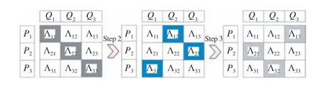
Fig.2. Handling segmentations and blocks in an HiDS matrix with DSGD.

For addressing this issue, data in an HiDS matrix should be rearranged to balance their distribution, making a DSGD algorithm achieve satisfactory speedup [38]. As shown in Fig.3(b), such a process is implemented by exchanging rows and columns in each segmentation at random [38].

C. Data Rearrangement Strategy MPSGD Algorithm

A momentum method is very efficient in accelerating the convergence rate of an SGD-based learning model [31], [33],[34]. It determines the learning update in the current iteration by building a linear combination of the current gradient and learning update in the last iteration. With such design,oscillations during a learning process decrease, making the resultant model converge faster. According to [33], with a momentum-incorporated SGD algorithm, the decision parameter θ of objective J(θ) is learnt as

Fig.3. Illustration of an MLF model.

In (4), Vθ(0)denotes the initial value of velocity, Vθ(t)denotes the t th iterative value of velocity, γ denotes the balancing constant that tunes the effects of the current gradient and previous update velocity, and o(t)denotes the t th training instance.

To build an SGD-based LF model, the velocity vector is updated at each single training instance. We adopt a velocity parameter v(P)m,kfor pm,kto record its update velocity, and thus generate V(P)|M|×dfor P. According to (4), we update pm,kfor single loss εm,non training instance rm,nas

Velocity constant γ in (5) adjusts the momentum effects.Similarly, we adopt a velocity parameter v(Q)n,kfor qn,kto record its update velocity, and thus V(Q)|N|×dis adopted for Q.The momentum-incorporated update rules for qn,kare given as

As depicted in Figs. 3(c)–(d) , with the momentumincorporated learning rules presented in (5) and (6), LF matrices P and Q can be trained with much fewer oscillations.Moreover, by integrating the principle of DSGD into the algorithm, we achieve an MPSGD algorithm that parallelizes the learning process of an LF model at high convergence rate.After dividing Λ into J data segmentations with J × J data blocks, we obtain

D. Data Rearrangement Strategy MPSGD Algorithm

With an MPSGD algorithm, we design Algorithm 1 for an MPSGD-based LF (MLF) model. Note that algorithm MLF further depends on the procedure update shown in Algorithm 2. To implement its efficient parallelization, we first rearrange Λ according to the strategy mentioned in Section III-B to balance Λ, as in line 5 of Algorithm 1. Afterwards, the rearranged Λ is divided into J data segmentations with J × J data blocks, as in line 6 of Algorithm 1. Considering the ith data segmentation, its j th data black is assigned to the jth training threads, as shown in lines 8−10 of Algorithm 1. Then all J training threads can be started simultaneously to execute procedure update, which addresses the parameter update related to its assigned data block with MPSGD discussed in Section III-C.

In Algorithm MLF, we introduce V(P)and V(Q)as auxiliary arrays for improving its computational efficiency. With J data segmentations and J training threads, each training thread actually takes 1/J of the whole data analysis task when the data distribution is balanced as shown in Fig.3(b). Thus, its time cost on a single training thread in each iteration is:

Therefore, its time cost in t iterations is:

* Note that all J training threads are started in parallel. Hence, the actual cost of this operation is decided by the thread consuming the most time.

A lgorithm 2 Procedure Update Operation 1for each rm,n in Λij//Cost: ×|Λ|/J 2 2 ˆrm,n=d∑ //Cost: Θ(d)3 for k = 1 to d do//Cost: × d 4 v(t)k=1 pm,kqn,k(P)m,k=γv(t−1)(P)m,k+η∂ε(t−1)m,n∂p(t−1)m,k //Cost: Θ(1)5 v(t)(Q)n,k=γv(t−1)(Q)n,k+η∂ε(t−1)m,n∂q(t−1)n,k //Cost: Θ(1)p(t)6 m,k ←p(t−1)m,k −v(t)(P)m,k //Cost: Θ(1)7 p(t)m,k ←p(t−1)m,k −v(t)(P)m,k //Cost: Θ(1)8 end for 9end for

Note that J−1, d and t in (8) and (9) are all positive constants, which result in a linear relationship between the computational cost of an MLF model and the number of known entries in the target HiDS matrix. However, owing to its parallel and fast converging mechanism, J−1and t can be reduced significantly, thereby greatly reducing its time cost.Next we validate its performance on several HiDS matrices generated by industrial applications.

IV. EXPERIMENTAL RESULTS AND ANALYSIS

A. General Settings

1) Evaluation Protocol: When analyzing an HiDS matrix from real applications [1]–[5], [7]–[10], [16], [19], a major motivation is to predict its missing data for achieving a complete relationship among all involved entities. Hence, this paper selects missing data estimation of an HiDS matrix as the evaluation protocol. More specifically, given Λ, such a task makes a tested model predict data in Γ. The outcome is validated on a validation set Ψ disjoint with Λ. For validating the prediction accuracy of a model, the root mean squared error (RMSE) and mean absolute error (MAE) are chosen as the metrics [9]–[11], [16], [37]–[39]

2) Datasets : Four HiDS matrices are adopted in the experiments, whose details are given below:

a) D1: Douban matrix. It is extracted from the China’s largest online music, book and movie database Douban [32].It has 16 830 839 ratings in the range of [1, 5] by 129 490 users on 58 541 items. Its data density is 0.22% only.

b) D2: Dating Agency matrix. It is collected by the online dating site LibimSeTi with 17 359 346 observed entries in the range of [1, 10]. It has 135 359 users and 168 791 profiles [11,12]. Its data density is 0.076% only.

c) D3: MovieLens 20M matrix. It is collected by the MovieLens site maintained by the GroupLens research team[37]. It has 20 000 263 known entries in [0.5, 5] among 26 744 movies and 138 493 users. Its density is 0.54% only.

d) D4: NetFlix matrix. It is collected by the Netflix business website. It contains 100 480 507 known entries in the range of[1, 5] by 2 649 429 users on 17 770 movies [11, 12]. Its density is 0.21% only.

e) All matrices are high-dimensional, extremely sparse and collected by industrial applications. Meanwhile, their data distributions are all highly imbalanced. Hence, results on them are highly representative.

The known data set of each matrix is randomly divided into five equal-sized, disjoint subsets to comply with the five-fold cross-validation settings, i.e., each time we choose four subsets as the training set Λ to train a model predicting the remaining one subset as the testing set Ψ. This process is sequentially repeated for five times to achieve the final results.The training process of a tested model terminates if i) the number of consumed iterations reaches the preset threshold,i.e., 1000, or ii) the error difference between two sequential iterations is smaller than the preset threshold, i.e., 10−5.

B. Comparison Results

The following models are included in our experiments:

M1: A DSGD-based LF model proposed in [30]. Note that M1’s parallelization is described in detail in Section III-A.However, it differs from an MLF model in two aspects: a) it does not adopt the data rearrangement as illustrated in Fig.3(b);and b) its learning algorithm is a standard SGD algorithm.

M2: An LF model adopting a modified DSGD scheme,where the data distribution of the target HiDS matrix is rearranged for improving its speedup with multiple training threads. However, its learning algorithm is a standard SGD algorithm.

M3: An MLF model proposed in this work.

With such design, we expect to see the accumulative effects of the acceleration strategies adopted by M3, i.e., the data rearrangement in Fig.3(b) and momentum effect in Fig.3(c).

To enable fair comparisons, we adopt the following settings:

1) For all models we adopt the same regularization coefficient, i.e., λP= λQ= 0.005 according to [12], [16].Considering the learning rate η and balancing constant γ, we tune them on one fold of each experiment to achieve the best performance of each model, and then adopt the same values on the remaining four folds to achieve the most objective results. Their values on each dataset are summarizes in Table I.

2) We adopt eight training threads for each model in all experiments following [29].

TABLE I PARAMETERS OF M1−M3 ON D1−D4

3) For M1−M3, on each dataset the same random arrays are adopted to initialize P and Q . Such a strategy can work compatibly with the five-fold cross validation settings to eliminate the biased results brought by the initial hypothesis of an LF model as discussed in [3].

4) The LF space dimension d is set at 20 uniformly in all experiments. We adopt this value to enable good balance between the representative learning ability and computational cost of an LF model, as in [3], [16], [29].

Training curves of M1−M3 on D1−D4 with training iteration count and time cost are respectively given in Figs. 4 and 5. Comparison results are recorded in Tables II and III.From them, we present our findings next.

a) Owing to an MPSGD algorithm, an MLF model converges much faster than DSGD-based LF models do. For instance, as recorded in Table II, M1 and M2 respectively take 461 and 463 iterations on average to achieve the lowest RMSE on D1. In comparison, M3 takes 112 iterations on average to converge on D1, which takes less than one fourth of that by M1 and M2. Meanwhile, M3 takes 110 iterations averagely to converge in MAE, which are also much less than 441 iterations by M1 and 448 iterations by M2. Similar results can also be observed on the other testing cases, as shown in Fig.4 and Tables II and III.

Meanwhile, we observe an interesting phenomenon that M1 and M2 converge at the same rate. Their training curves almost overlap on all testing cases according to Fig.4. Note that M2 adopts the data shuffling strategy mentioned in Section III-A as in [30] to balance the known data distribution of an HiDS matrix distribute uniformly while M1 does not.This phenomenon indicates that the data shuffling strategy barely affects the convergence rate or representative learning ability of an LF model.

b) With an MPSGD algorithm, an MLF model’s time cost is significantly lower than those of its peers. For instance, as shown in Table II, M3 averagely takes 89 s to converge in RMSE on D3. In comparison, M1 takes 1208 s, which is over 13 times M3’s time. M2 takes 308 s, which is still over three times M3’s average time. The situation is the same with MAE as the metric, as recorded in Table III.

c) Prediction accuracy of an MLF model is comparable with or slightly higher than those of its peers. As recorded in Tables II and III, on all testing cases M3’s prediction error is as low as or even slightly lower than those of M1 and M2.Hence, an MPSGD algorithm can slightly improve an MLF model’s prediction accuracy for missing data of an HiDS matrix as well as its high computational efficiency.

d) The stability of M1−M3 are close. According to Tables I and II, we see that the standard deviations of M1−M3 in MAE and

RMSE are very close on all testing cases. Considering their time cost, since M1 and M2 generally consume much more time than M3 does, their standard deviations in total time cost are generally larger than that of M3. However, it is also datadependent. On D4, we see that M1−M3 have very similar standard deviations in total time. Hence, we reasonably conclude that two acceleration strategies, i.e., data rearrangement and momentum-incorporation, do not affect its performance stability.

C. Speedup Comparison

A parallel model’s speedup measures its efficiency gain with the deployed core count, i.e.,

where T1and TJdenote the training time of a parallel model deployed on one and J training threads, respectively. High speedup of a parallel model indicates its high scalability and feasibility for large-scale industrial applications.

Fig.4. Training curves of M1−M3 in iteration count. All panels share the legend of panel (a).

Fig.5. Training curves of M1−M3 in time cost. All panels share the legend of panel (a).

TABLE II PERFORMANCE COMPARISON AMONG M1−M3 ON D1−D4 WITH RMSE AS AN ACCURACY METRIC

TABLE III PERFORMANCE COMPARISON AMONG M1−M3 ON D1−D4 WITH MAE AS AN ACCURACY METRIC

Fig.6. Parallel performance comparison among M1−M3 as core count increases. Both panels share the legend in panel (a).

The speedup of M1−M3 on D4 as J increases from two to eight is depicted in Fig.6. Note that similar situations are found on D1−D3. From it, we clearly see that M3, i.e., the proposed MLF model, outperforms its peers in achieving higher speedup. As J increases, M3 always consumes less time than its peers do, and its speedup is always higher than those of its peers. For instance, from Fig.6(b) we see that M3’s speedup as J = 8 is 6.88, which is much higher than 4.61 by M1 and 4.44 by M2. Therefore, its scalability is higher than those of its peers, making it more feasible for real applications.

D. Summary

Based on the above results, we conclude that:

a) Owing to an MPSGD algorithm, an MLF model has significantly higher computational efficiency than its peers do;and

b) An MLF model’s speedup is also significantly higher than that of its peers. Thus, it has higher scalability for large scale industrial applications than its peers do.

V. CONCLUSIONS

This paper presents an MLF model able to perform LF analysis of an HiDS matrix with high computational efficiency and scalability. Its principle is two-fold: a) reducing its time cost per iteration through balanced data segmentation,and b) reducing its converging iteration count by incorporating momentum effects into its learning process.Empirical studies show that compared with state-of-the-art parallel LF models, it has obviously higher efficiency and scalability in handing an HiDS matrix.

Although an MLF model performs LF analysis on a static HiDS matrix with high efficiency, its performance on dynamic data [12] remains unknown. As discussed in [41], a GPU-based acceleration scheme is highly efficient when manipulating full matrices in context of recommender systems and other applications [42]–[50]. Nonetheless, more efforts are required to adjust its fundamental matrix operations to be compatible with an HiDS one as concerned in this paper. We plan to address these issues in the future.