Investigation of hypersonic flows through a cavity with sweepback angle in near space using the DSMC method*

Guangming Guo(郭广明), Hao Chen(陈浩), Lin Zhu(朱林), and Yixiang Bian(边义祥)

College of Mechanical Engineering,Yangzhou University,Yangzhou 225127,China

Keywords: flow characteristics,cavity with sweepback angle,hypersonic flow,near space,DSMC

1. Introduction

The scramjet(supersonic combustion ramjet)is an innovative engine for airbreathing hypersonic vehicles and it would become one of the most effective engines for the hypersonic flight in the near future.[1]However, the main obstacle in the realization of such objective is the quite low mixing efficiency between the injected fuel and air due to the very short residence time of the fuel inside the combustor.[2]In order to promote the mixing process between the fuel and air,a variety of devices,as outlined in Refs.[3,4],are designed in recent years to enhance the mixing,such as ramp,[5]aerodynamic ramp,[6]strut,[7]and cavity.[8]Among these devices, the cavity acting as the flame holder has been widely used in the scramjet engine to prolong the residence time of fuel at supersonic/hypersonic conditions.[9]For this reason, the cavities with different configurations have been investigated numerically and experimentally by many researchers.[2,10-15]

Huang[2]investigated the influence of cavity configuration on the combustion flow field performance of the hypersonic vehicle,and found that the cavity with a sweptback angle of 45°could further improve the aero-propulsive performance of the hypersonic vehicle. He also investigated the influence of geometric parameters on the drag force of the heated flow field around the cavity by variance analysis method.[13]Vinha studied the incompressible fluid flow over a rectangular open cavity for understanding the evolution of the span-wise instabilities of flow and interaction between different dynamic modes with the dynamic mode decomposition algorithm.[10]The characteristics of the cavities with different shapes in the freestream with low velocity were experimentally tested by Ozalp.[11]Luo[12]estimated and compared the drag forces of three different geometric configurations of the cavity flame holder, namely the classical rectangular, triangular and semicircular,and the cavities were with the fixed depth and lengthto-depth ratio. He found that the triangular cavity imposes the most additional drag force on the scramjet engine,and the drag force of the classical rectangular one is the least.

Near space is generally defined as the region between 20 and 100 km of the atmosphere,including a majority of regions in the stratosphere, the mesosphere and partial regions in the thermosphere,[16]and it has been paid more and more attention in recent years due to its military application value. The flying vehicles in near space usually have hypersonic speeds (i.e.,M∞≥5), namely the hypersonic vehicles. For example, the hypersonic cruise vehicle concept in the Falcon program has a cruise Mach number of 10.[17]Gerdroodbary[18]simulated a 2D axisymmetric aero-disked nose cone in hypersonic flow ofM∞=5.75 at 0°angle of attack, with and without gas injection,and the numerical results showed that high-speed vehicle design and performance can benefit from the application of counter-flowing jets as a cooling system. Flow parameters and skin temperature distributions caused by aerodynamic heating were simulated and analyzed by Murty for a high speed(～5Ma) aerospace vehicle at about 25 km using commercial CFD code.[19]However, according to the published papers, the study on cavity configuration for hypersonic speeds in near space has rarely been investigated, probably because of the difficulties in experimentally measuring reliable data at hypersonic condition and the rarefied gas effects in near space,which motivates the current work.

The purpose of this work is to explore flow characteristics of a hypersonic cavity with sweepback angle in near space under different conditions by using the direct simulation Monte Carlo (DSMC) method, which is one of the most successful particle methods in treating rarefied gas dynamics.[20]The rest of this paper is organized as follows: the DSMC method is introduced and validated in Section 2;computational configuration,simulation cases,and grid independence are described in Section 3; simulation results of the considered cases and discussion are presented in Section 4; some significant conclusions drawn from this work are given in Section 5.

2. Numerical method and code validation

2.1. DSMC introduction

The Boltzmann equation is able to describe the flow behavior of gas at every rarefaction degree and it can be solved by stochastic schemes, commonly known as DSMC.In short, the DSMC method is a particle based microscopic method that converges to the solution of the Boltzmann equation in the limit of infinite simulating particles and cells.[20]In this method, simulating particles represent a cloud of gas molecules that travel and collide with each other and solid surfaces. The macroscopic properties of the gas such as velocity,temperature, density, shear stress, and pressure are obtained by taking appropriate sampling of microscopic properties of the simulating particles after the flow field is stable.

Over the past few decades, the DSMC method has become the predominant predictive tool in rarefied and lowdensity gas flows. However, computational consumption is probably the main blockage factor existing in the extensive application of DSMC method. Generally speaking, there are two different ways to solve this difficulty when facing massive computation. One way is to improve the DSMC method,such as with MPC algorithm,[21]or asymptotic-preserving(AP) algorithm.[22]The other way is to introduce some assistant techniques such as the efficient parallel technology,[23]which is used in current DSMC code. For numerical simulation, mathematical modeling is critical for obtaining reliable results.[24,25]See Refs. [26-32] for the details of our DSMC method.

In this work, the parallel DSMC code in which the variable hard sphere (VHS) model and no-time-count collision(NTC) scheme are used to simulate the molecular collisions.The parallel load identification of the code is based on the number of simulating particles and collision number per cell.The general Larsen-Borgnakke model is used to redistribute the rotational energy during the translational-rotational (TR) energy transfer. Before this, it needs to perform the translational-vibrational (T-V) energy transfer to redistribute the vibrational energy using the quantum Larsen-Borgnakke model with the harmonic oscillator model. The rotational collision number is set to 10, and the vibrational collision number is set to 100. According to our experience in DSMC simulations, the sampling times after the cavity steady flow is set to 20000 for a sufficiently small statistical error and it uses 20 simulating particles per cell to reduce the influence of statistical dependence, and then the statistical error, which is inversely proportional to the square root from the product of sampling times and simulating particles per cell, is about 1.0%. Because the DSMC simulation is sensitive to the grid resolution, the cell size in each simulation case of this work is less than one-third of the local mean free path(MFP).The time step is not a constant but varies with the altitude.

2.2. Validation of the DSMC code

In order to verify the validity of our DSMC code in simulating hypersonic cavity flow in near space,the cavity with a length-to-depth ratio of 4 and under a freestream Mach number of 25 at the altitude of 70 km is used to carry out the DSMC code, and the detailed flow conditions are listed in Table 1 of Ref. [33]. Figure 1 shows the streamline patterns and dimensionless normal velocity inside the cavity of the current DSMC results and those presented in Ref.[33],where the three dimensionless normal velocity profiles are plotted with the data extracted from the three transversal sections defined by the dimensionless height ofy=0.25H, 0.5H, and 0.75H,respectively.The comparison of streamline patterns inside and around the cavity is displayed by Figs. 1(a) and 11(b), it is evident that both the two separated corner vortices and the streamlines of the current DSMC simulation and Palharini are rather similar to each other. In addition, it is observed that the three dimensionless normal velocity profiles of the current DSMC simulation have a very close agreement with those of Palharini,as presented in Fig.1(c). On the whole,the comparison shown in Fig.1 provides a good supportive evidence for the simulation accuracy of our DSMC code.

Fig.1. Comparison between streamline patterns and dimensionless normal velocity inside the cavity:streamline patterns of(a)Palharini and(b)the current DSMC simulation,and(c)dimensionless normal velocity.

3. Computational configuration, simulation cases and grid independency analysis

3.1. Computational configuration

The flow over a cavity will be approximately symmetrical concerning the central plane of the cavity if the aspect ratio of the cavity is large enough. In addition,considering the computation cost of the DSMC method, this study is only a theoretical exploration,and the 2D cavity flow is investigated in this work. Sketch map of the computational domain for the cavity with sweepback angle is presented in Fig. 2. The depth (H) and length (L) of the cavity is 10 and 50 mm, respectively,so the length-to-depth ratio is 5.0. The sweepback angle (θ) of the cavity is a variable parameter and it is set to be 30°,45°,60°,and 90°in this study. The lengths of the upstream and downstream walls are 30 and 20 mm,respectively,and the height of the computational domain is 15 mm for both upstream inlet and downstream outlet. The origin of coordinate system employed in this paper is located at the lower left corner of the cavity, andxandydenote the streamwise and vertical directions,respectively.

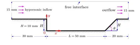
Fig.2. Sketch map of the computational domain for the cavity configuration.

3.2. Simulation cases

In this subsection, some simulation cases with different purposes are designed to reveal flow characteristics of the cavity configuration in near space. For example, for the cavity with a sweepback angle of 45°,the altitude(A)of 20-60 km is considered to reveal the influence of altitude on flow characteristics(see Table 1). In addition,the freestream Mach number(Ma∞) of 10, 15, and 20 (see Table 2) and sweepback angle of ranging from 30°to 90°(see Table 3)are used to reveal the influence on flow characteristics.

Table 1. Computational conditions of the cavity at different altitudes.

Table 3. Computational conditions of the cavity with different sweepback angles.

Because the freestream flows from left to right (see Fig. 2), the inlet boundary condition is imposed on the left border of the computational domain, and the right border of the computational domain is flow outlet. The upper border of the computational domain is free interface and the remaining borders are walls where the no slip, impenetrable and constant temperature conditions are adopted. The freestream consists of 78%N2and 22%O2and its molecular weight is about 28.96 kg/mol.The freestream pressure(P∞),temperature(T∞),and density(ρ∞)are consistent with those of the corresponding environment conditions.

It should be pointed out that, from these altitudes in Table 1,the flow regime belongs to continuum or near-continuum according to the freestream Knudsen number. In the cavity,however,the local Knudsen number,which is generally used to describe the level of rarefaction effect,is usually much larger than the freestream Knudsen number. For example, the maximum local Knudsen number within the cavity is about 7 and 16 times as large as the freestream Knudsen number for the Case 2 and Case 4, respectively. It is generally considered that the flow is outside the continuum regime when the local Knudsen number is greater than 0.05,[34]namely,the local rarefaction effect can not be ignored under this condition,and therefore it is necessary to use the DSMC method to carry out this work.

3.3. Grid independence analysis

The calculation precision of the DSMC method is mainly determined by grid density, times of sampling, particle number in each mesh cell and time step. As stated in the Subsection 2.1,the times of sampling,particle number in each mesh cell,and time step are set to appropriate values to ensure simulation accuracy of the DSMC method,and thus only the grid density (i.e., grid independence) is discussed in this subsection.

The Case 2 listed in Table 1 is used to assess grid independence with three levels of grid refinement: coarse grid(98000 mesh cells), moderate grid (270000 mesh cells) and fine grid (390000 mesh cells), and these grids are generated using the commercial software POINTWISE. As shown in Fig.3, the computational grid is densely clustered near walls of the cavity, at the entrance of freestream, in the vicinity of the step and trailing edge,and in the shear flow area. It should be noted that most of the grid points are skipped in Fig.3 for the purpose of clarity.

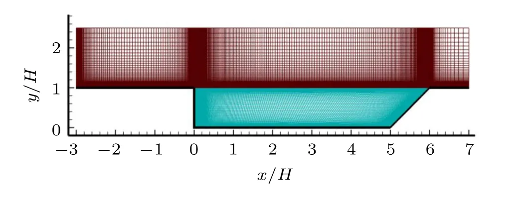
Fig.3. An example of computational grid for the cavity configuration.

Figure 4 shows streamwise velocity and density distribution along the vertical line ofx/H=3 for these three computational grids. It is found that deviation of streamwise velocity and density is slight for different grids, especially for the moderate and fine grids. The moderate grid is reasonable considering computational cost of the DSMC method, and thus grid refinement as that of the moderate grid is adopted for the computational grids used in the following DSMC simulations.

Fig. 4. Comparison of streamwise velocity (left) and density (right) along the vertical line of x/H =3 for three different grid densities to test the grid independence.

4. Results and discussion

4.1. Features of the flow field

The Case 1 listed in Table 1 is simulated and analyzed here to show basic features of the cavity flow in near space,which is helpful in understanding the subsequent subsections better. Figure 5 displays velocity contours of the flow field and velocity profiles inside three typical areas,namely,the upstream and downstream boundary layers and the shear layer formed at the step edge. For the upstream boundary layer(see A1), theMaprofile along the vertical line ofx/H=-2 indicates that the velocity almost increases linearly within the boundary layer defined based on the 99% freestream velocity criterion,[24]whereas it increases sharply near the border of the boundary layer. Similarly, velocity in the downstream boundary layer has the same feature,see theMaprofile along the vertical line ofx/H=6.5.For the shear layer(see A2),theMaprofiles along the vertical lines ofx/H=0.732,1.588,and 2.505 are similar and they are all approximately symmetrical concerning the point ofMa=3,which is the theoretical convection speed of the shear layer.[35]That is, the whole shear layer marked by two white dotted lines moves downstream at an average speed ofMa=3. It is also observed that the shear layer spans the entire cavity length and this is consistent with the flow feature of an open cavity.

Fig. 5. Velocity contour of the flow field (top) and velocity profiles in three typical areas (bottom) Note: minus sign of the Mach number only indicates the flow direction.

In order to reveal flow patterns inside the cavity,streamline of the flow field is shown in Fig.6. It is seen that a large vortex, which forms the primary recirculation region of occupying the most area of the cavity, and the smaller vortex located at the lower left corner of the cavity forms the secondary recirculation region underneath the primary recirculation region. As indicated in Fig. 6, both the primary and secondary recirculation regions have a smaller accompanied vortex which has the same rotation direction with that of its corresponding recirculation region. Specifically, the primary recirculation region rotates clockwise because it is induced by the freestream,whereas the secondary recirculation region rotates anticlockwise because it is derived from the primary recirculation region. That is,the secondary recirculation region is driven by the primary recirculation region.

Fig.6. Streamline of the flow field for Case 1.

Figure 7 displays the pressure contour of the flow field,where the leading-edge shock wave (labeled 1○), expansion wave formed at the step edge (labeled 2○), low-pressure area(labeled 3○)defined as the area in which the pressure is smaller than that of the freestream, and the compression-expansion wave area (labeled 4○) are shown clearly. The isobars in areas 3○and 4○are given in the bottom of Fig.7 to reveal pressure feature in the both areas and meanwhile, the streamlines are also displayed. For the low-pressure area (see 3○), it is seen that the isobars in the primary recirculation region are nearly centre-symmetrical concerning the core of the primary recirculation region,and the pressure becomes lower as it approaches to the vortex core. It is also observed that the pressure distribution in the primary recirculation region is stratified due to circular motion of the fluid inside the primary recirculation region. For the compression-expansion wave area (see 4○), it is found that the pressure increases significantly along the ramp wall until it arrives at the peak of the ramp(namely,the trailing edge of the cavity), while the pressure decreases quickly when it leaves from the trailing edge to the downstream. Also, it is found that the maximal pressure nearby the trailing edge is about five times larger than that of the freestream.

Figure 8 shows the temperature contours of the flow field and there are two high-temperature areas, among which, one exists in the primary recirculation region(labeled B3)and the other is nearby the trailing edge of the cavity(labeled B1),and a low-temperature area located in the left side of the cavity(labeled B2). In order to reveal the temperature feature in these three areas,the isotherms along with streamlines in each area are displayed in the bottom of Fig.8.For the high-temperature area B3, it is clear that the shape of each isotherm is like an ellipse as that of the streamline,and the temperature becomes larger as it approaches to the vortex core. That is,the temperature distribution in the primary recirculation region is stratified due to circular motion of the fluid in this region. For the hightemperature area B1,there is a maximum temperature nearby the trailing edge of the cavity because of intense interaction between hypersonic freestream and the wall around it,whereas the temperature downstream of the trailing edge decreases due to the decreasing interaction.For the low-temperature area B2,the stratification phenomenon of temperature distribution disappears because the flow velocity of fluid in this area is low(see Fig. 5), and the temperature variation in this area is not significant.

Fig.7. Pressure contours of the flow field for Case 1.

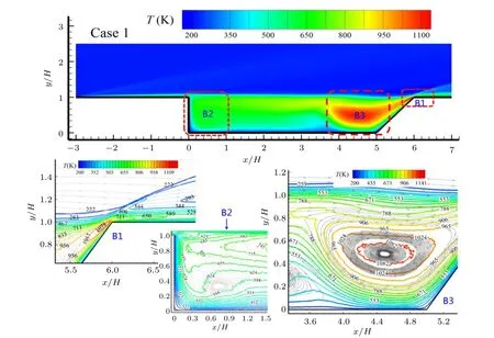
Fig.8. Temperature contours of the flow field for Case 1.

4.2. Influence of different altitudes

Due to the rarefied gas effects in the near space,flow characteristics of the cavity would highly depend on altitude. In this subsection, the altitudes of 30, 40, and 60 km are taken into account to explore the evolution of the cavity flow with altitude. Figure 9 compares velocity contours and streamlines of the flow field for various altitudes.Specifically,for the comparison of the velocity contours, two obvious features can be found. First,an increase in altitude would lead to an increase in thickness of the upstream and downstream boundary layers and the shear layer,and the increment is especially significant for Case 4. For example, the shear layer of Case 4 is quite thick and nearly touches the bottom of the cavity, the downstream boundary layer(i.e.,x/H ＞6)is essentially the continuation of the shear layer, which is quite different from those of Cases 2 and 3. Second, flow velocity in the secondary recirculation region increases with the increasing altitude. For the comparison of streamlines,some distinct changes are also observed such as the number of vortices inside the cavity decreases from four in Cases 2 and 3 to two in Case 4 as the altitude increases. Because of extrusion effect from the expanded shear layer (see Case 4), the primary and secondary recirculation regions are pushed to the right and left corners of the cavity,respectively.

As analyzed above, the secondary recirculation region is induced by the primary recirculation region at low altitudes(e.g.,Cases 1,2,and 3),whereas it is driven by the expanded shear layer at the higher altitude (e.g., Case 4). As a result,rotation direction of the secondary recirculation region is reversed at different altitudes, as illustrated in Fig. 10. However, rotation direction of the primary recirculation region is the same for each altitude because it is always derived by the hypersonic freestream.

The comparison of pressure contours of the flow field for various altitudes is displayed in Fig. 11, it is clear that the pressure decreases greatly with the increase of altitude. For the three cases,a strong compression-expansion wave formed around the trailing edge of the cavity, a shock wave generating in the leading edge, and both of them become much weaker and diffuse distinctly with the increasing altitude.Meanwhile, the low-pressure area within the cavity that marked by a white ring moves away from the primary recirculation region to the secondary recirculation region.

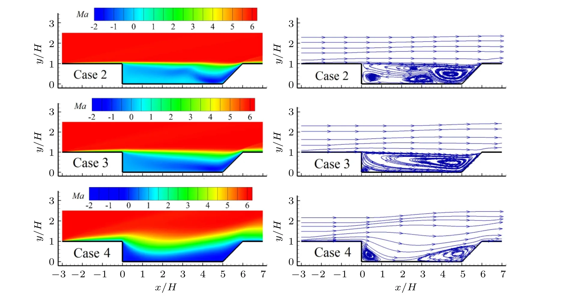
Fig.9. Comparison of the velocity contours(left)and the streamlines(right)of the flow field for various altitudes. Note: minus sign of the Mach number only indicates the flow direction.

Fig.10. Comparison of rotation direction of the secondary recirculation region: (left)Case 2 and(right)Case 4.

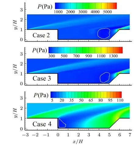
Fig. 11. Comparison of the pressure contours of the flow field for various altitudes.

In order to reveal distribution feature of pressure inside the cavity,pressure profiles along the horizontal line ofy/H=0.5 and downstream wall of the cavity for various altitudes are extracted and given in Fig. 12, where the pressure has been normalized with that of the freestream. For Cases 2 and 3,it is found that pressure on the horizontal line ofy/H=0.5 is approximately constant and it is slightly lower than that of the freestream until it is in the primary recirculation region,in which the pressure reduces further.For Case 4,the pressure almost increases linearly on the whole line. The reason why the pressure inside the cavity varies remarkably in Case 4 is probably that the shear layer intrudes into the cavity (see Fig. 9),which results in acceleration of the fluid inside the cavity and reversion of the rotation direction of the secondary recirculation region.

The pressure distribution along downstream wall of the cavity has a similar feature for various altitudes,see the right of Fig.12. Specifically,the pressure increases quickly due to fluid compression before the trailing edge of the cavity and after the trailing edge,the pressure decreases sharply because of fluid expansion. The maximum pressure nearby the trailing edge is about 4.4,3.9,and 3.8 times larger than that of the freestream for Cases 2,3,and 4,respectively.

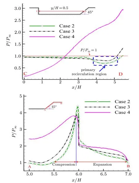
Fig.12.Pressure profiles along the horizontal line of y/H=0.5(i.e.,C→D)and downstream wall(i.e.,A→B)of the cavity for various altitudes. Note:the pressure is normalized with that of freestream.

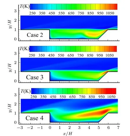
Fig. 13. Comparison of temperature contours of the flow field for various altitudes.

As shown in Fig. 13, the high-temperature area enlarges remarkably with the increasing altitude, its shape is like a sloped strip for Case 4 while it is like an ellipse for Case 2,and this implies that formation mechanism of the high-temperature area is different for the two cases. As a matter of fact,the high-temperature area of Case 2 is induced by the primary recirculation region, while it is formed due to the expanded shear layer in Case 4. Another notable phenomenon is that the maximum temperature departs from the trailing edge of the cavity with the increase of altitude. Taking Case 4 for example,the expanded shear layer pushes the high-temperature area away from the trailing edge,and thus the maximum temperature nearby the trailing edge reduces greatly compared with those of Cases 2 and 3, as illustrated in Fig. 14. It is observed that the maximum temperature nearby the trailing edge is about 1150,1060,and 540 K for Cases 2,3,and 4,respectively.

Fig.14. Temperature profiles along the downstream wall(i.e.,A→B)of the cavity for various altitudes.

4.3. Influence of different Mach numbers

The Mach number is an important flight parameter for an aerospace vehicle and some high Mach numbers such as 10,15, and 20 are used to reveal the influence of Mach number on cavity flow characteristics in near space. Figure 15 compares the velocity contours and streamlines of the flow field for various Mach numbers. With the increase of Mach number,the downstream boundary layer becomes thicker gradually while the upstream boundary layer and shear layer seem to be changeless. Also,it is observed that the primary recirculation region is gradually enlarged with Mach number,and it nearly occupies the whole cavity in Case 7. Consequently, the secondary recirculation region is driven further toward the lower left corner of the cavity and meanwhile it becomes smaller gradually.

Figure 16 shows comparison of the pressure contours of the flow field for various Mach numbers and an obvious feature is that the low-pressure area marked by white ring within the cavity disappears gradually with the increase of Mach number. In order to reveal distribution feature of pressure inside the cavity, pressure profiles along the horizontal line ofy/H=0.5 and downstream wall of the cavity for various Mach numbers are extracted and shown in Fig. 17, where the pressure has been normalized with that of freestream. It is found that each profile has a similar shape for both the horizontal line and the downstream wall and the pressure increases gradually with the increase of Mach number. For pressure distribution along the downstream wall of the cavity,there is a sharp drop nearby the trailing edge because of the compression-expansion shock wave conversion. The maximum pressure nearby the trailing edge is about 6.1,5.0,and 4.95 times larger than that of freestream for Cases 7,6,and 5,respectively.

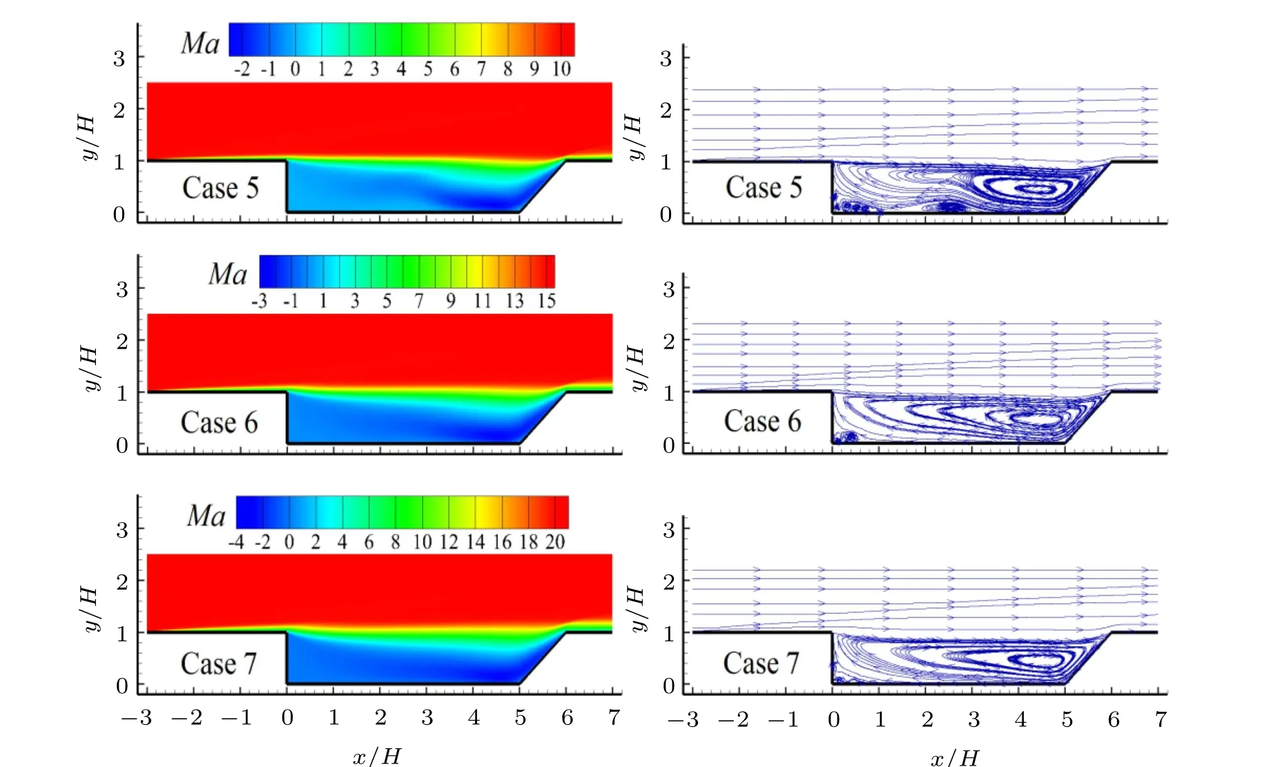
Fig.15. Comparison of velocity contours(left)and streamlines(right)of the flow field for various Mach numbers. Note: minus sign of the Mach number only indicates the flow direction.

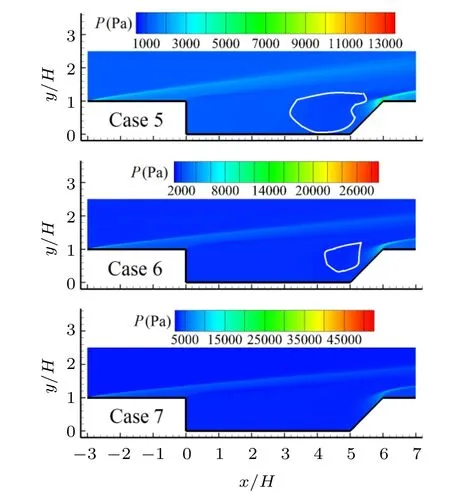
Fig.16. Comparison of pressure contour of the flow field for various Mach numbers.

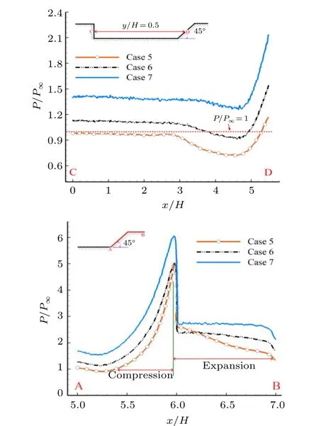
Fig.17.Pressure profiles along the horizontal line of y/H=0.5(i.e.,C→D)and downstream wall(i.e.,A→B)of the cavity for various Mach numbers.Note: the pressure is normalized with that of freestream.

As shown in Fig. 18, the temperature in the cavity increases greatly with the increase of Mach number, the maximum temperature is always located at the location nearby the trailing edge, the temperature of fluid in the primary recirculation region is high,while the temperature of fluid in the secondary recirculation region is quite low. The specific temperature value along the downstream wall of the cavity is given in Fig.19,it is seen that the maximum temperature nearby the trailing edge is about 2400 K,4030 K,and 6120 K for Cases 5,6,and 7,respectively,which indicates that Mach number has a significant influence on temperature of fluid within the cavity.

Fig. 18. Comparison of temperature contour of the flow field for various Mach numbers.

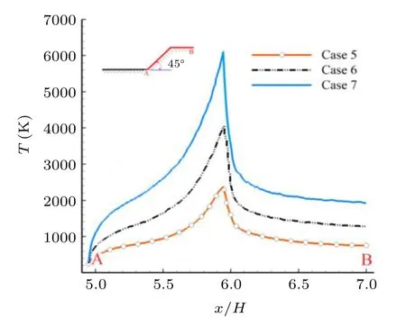
Fig.19. Temperature profiles along the downstream wall(i.e.,A→B)of the cavity for various Mach numbers.

4.4. Influence of different sweepback angles

The sweepback angle is an important factor for the cavity and it is usually used to optimize aero-propulsive performance.[15]In this subsection, the sweepback angle is acted as a variable to investigate its impact on the flow characteristics, and its values such as 30°, 60°, and 90°are taken into account. The comparison of the velocity contours and the streamlines of the flow field for various sweepback angles are given in Fig.20. As expected,the sweepback angle has a significant influence on the flow within the cavity. First,the shear layer becomes thinner gradually with the sweepback angle increases and meanwhile it is lifted by the primary recirculation region. Second,the number of vortices inside the cavity varies from two for the sweepback angle of 30°to four for the sweepback angles of 60°and 90°. Third,the larger vortex in the primary recirculation region shrinks distinctly with the increase of sweepback angle and meanwhile, the secondary recirculation region further reduces because of extrusion effect from the primary recirculation region.

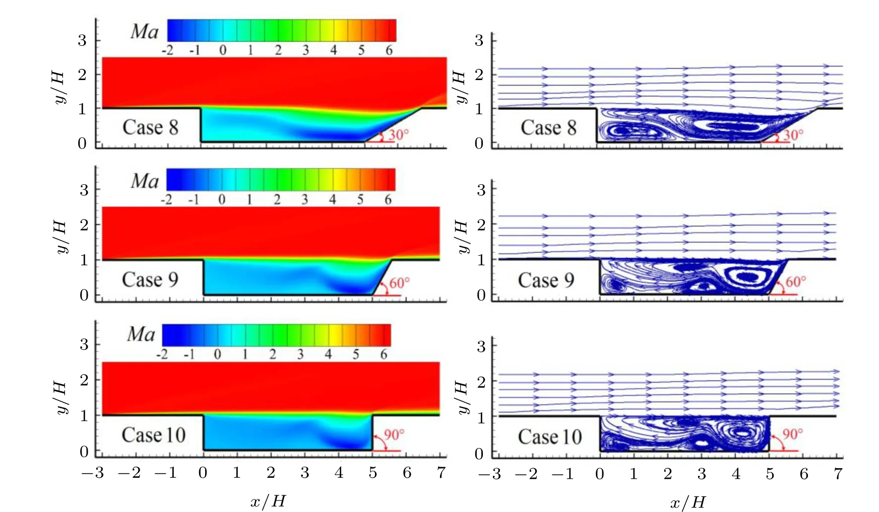
Fig.20. Comparison of velocity contours(left)and streamlines(right)of the flow field for various sweepback angles. Note:minus sign of the Mach number only indicates the flow direction.

Fig.21. Comparison of pressure contour of the flow field for various sweepback angles.

Fig.22.Pressure profiles along the horizontal line of y/H=0.5(i.e.,C→D)and downstream wall (i.e., A→B) of the cavity for various sweepback angles. Note: the pressure is normalized with that of freestream.

Figure 21 compares pressure contours of the flow field for various sweepback angles and a notable feature is that the lowpressure area marked by the white ring in the cavity reduces gradually,and the pressure distribution in the upstream of the flow field seems to be not affected by these sweepback angles.In order to show distribution feature of pressure inside the cavity quantitatively,pressure profiles along the horizontal line ofy/H=0.5 and downstream wall of the cavity for various sweepback angles are extracted and given in Fig. 22, where the pressure has been normalized with that of freestream. It is observed that the pressure profile is approximately constant except in the primary recirculation region where it is like a U-type curve due to vortex flow in the primary recirculation region. In addition,the pressure increases with the increase of sweepback angle. On the contrary, the pressure at the downstream wall of the cavity decreases quickly with the increase of sweepback angle, the maximum pressure nearby the trailing edge is about 7.6, 3.6, and 2.9 times larger than that of freestream for the sweepback angle of 30°, 60°, and 90°, respectively, and the mechanism for this situation can be illustrated by Fig.23. For the sweepback angle of 30°,the hypersonic freestream directly strikes the wall nearby the trailing edge and thus it produces a great impact force on the wall.With the increase of sweepback angle,the freestream over the cavity floor is lifted by the primary recirculation region and it is no longer hit the wall nearby the trailing edge,which leads to a significant reduction of the impact force. Consequently,the pressure reduces greatly with the increase of sweepback angle,as shown in the right of Fig.22.

Fig.23. Isobars and streamline of the flow field around the trailing edge of cavity for various sweepback angles.

The comparison of temperature contours of the flow field for various sweepback angles is displayed in Fig.24. It is seen that the high-temperature area inside the cavity shrinks obviously with the increase of sweepback angle and meanwhile a waved low-temperature area emerges gradually near the cavity floor, as shown by the white curves in Fig.24. The temperature profile along the downstream wall of the cavity is shown in Fig. 25 and the maximum temperature nearby the trailing edge is about 1130,1080,and 1010 K for Cases 8,9,and 10,respectively, which indicates that the sweepback angle has a weak influence on maximum temperature in the flow field.

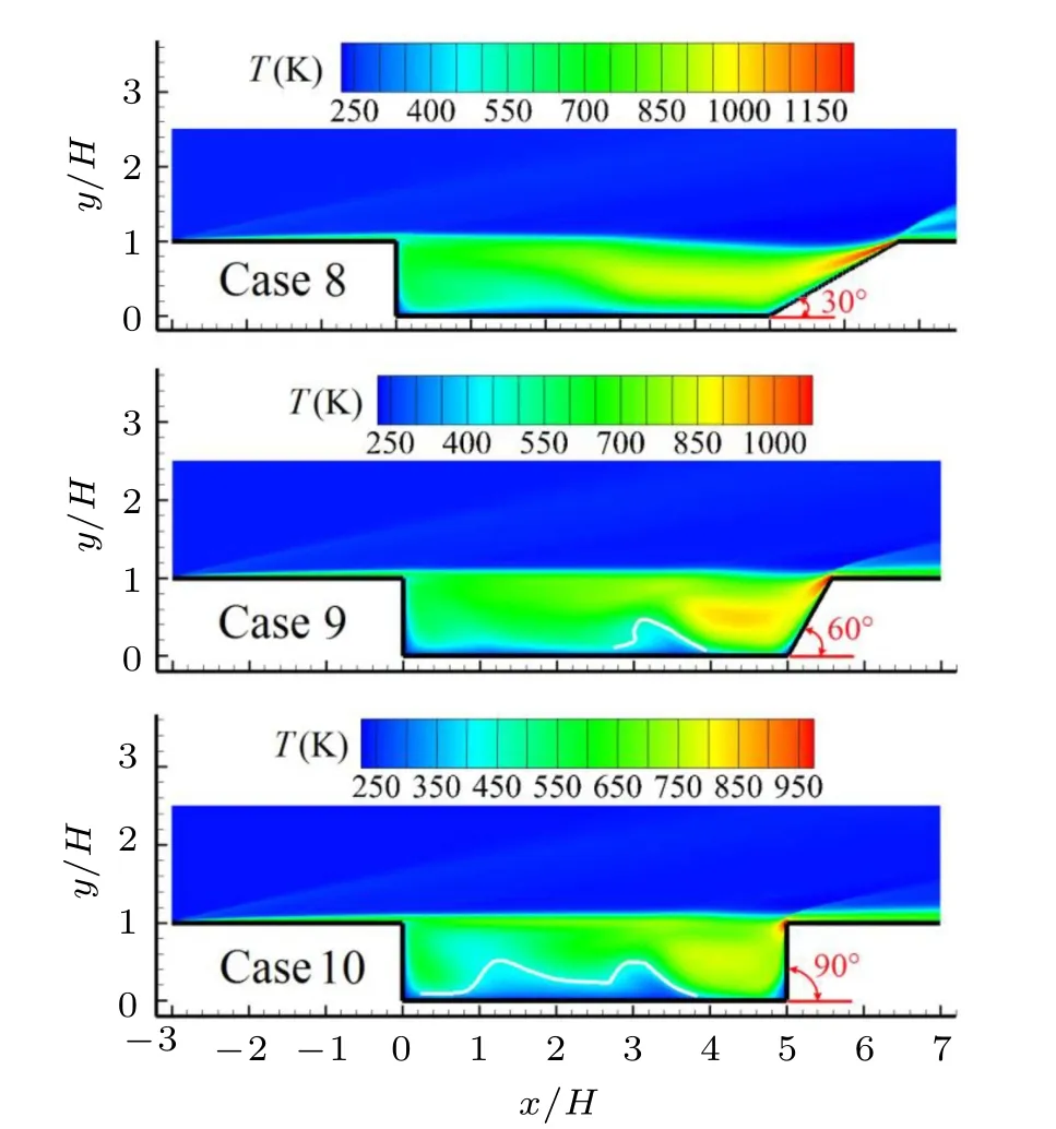
Fig. 24. Comparison of temperature contours of the flow field for various sweepback angles.

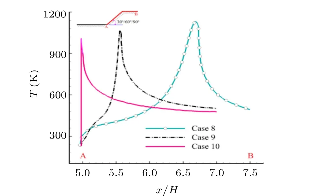
Fig.25. Temperature profiles along the downstream wall(i.e.,A→B)of the cavity for various sweepback angles.

5. Conclusions

The DSMCmethod has been employed to explore flow characteristics of a cavity with sweepback angle in near space by considering the cases such as the altitude of 20-60 km,the Mach number of 6-20, and the sweepback angle of 30°-90°.Summarizing this work,the following conclusions can be drawn:

1) The primary and secondary recirculation regions are the main flow structures in the cavity, both the low-pressure and high-temperature areas are formed in the primary recirculation region,and distribution of the pressure and temperature in the primary recirculation region is stratified.

2)The shear layer becomes bent and invades the interior of the cavity with the increase of altitude, leading to the separation of the primary recirculation region and the secondary recirculation region, and pushing them to the lower right and left corners of the cavity respectively. A notable finding is that the rotation direction of the secondary recirculation region is reversed at a higher altitude due to the change of formation mechanism of the secondary recirculation region. For the primary recirculation region,however,its rotation direction is always the same for various altitudes.

3)The velocity,pressure,and temperature of fluid within the cavity increase, the primary recirculation region enlarges while the secondary recirculation region reduces with the increase of Mach number, and a noteworthy feature is that the low-pressure area in the cavity disappears gradually.

4)With the increase of sweepback angle,the shear layer becomes thinner gradually and meanwhile it is lifted by the primary recirculation region, the secondary recirculation region reduces further, and both the high-temperature and lowpressure area reduce due to shrinkage of the primary recirculation region. Moreover,a waved low-temperature area emerges gradually near the cavity floor, and the maximum pressure nearby trailing edge of the cavity decreases sharply.

Acknowledgements

The authors thank the Prof. H. Liu’s team of Shanghai Jiao Tong University for providing the DSMC code for this research. Also,the first author thanks the Program for Innovative and Entrepreneurial Talents in Jiangsu Province.