
Transition to chaos in lid–driven square cavity flow∗
2021-12-22 06:47TaoWang王涛andTiegangLiu刘铁钢
Chinese Physics B 2021年12期
关键词:王涛
Tao Wang(王涛) and Tiegang Liu(刘铁钢)
1School of Mathematics and Information Science,North Minzu University,Yinchuan 750021,China
2LMIB and School of Mathematical Sciences,Beihang University,Beijing 100191,China
Keywords: unsteady lid–driven square cavity flows,chaos,time series analysis,third Hopf bifurcation
1. Introduction
In the past 60 years, research into two-dimensional(2D)flows in a lid–driven square cavity has been regarded as a benchmark study.[1–6]The shape of this model makes it relatively simple to validate the accuracy and reliability of new methods by comparison with the benchmark solution.
In recent decades,researchers have shifted research focus to studying the Hopf bifurcations. The early studies on Hopf bifurcation mainly focused on the first bifurcation, in which the flow transfers its stationary state to a non-stationary periodic state. In a former work,[3]it was suggested that the first Hopf bifurcation occurs when the critical Reynolds number ofRec1is larger than 7500. Since then various results have been given. It has been given as aboutRec1=7763±2%,[7]close toRec1=8000[8]or greater than 8000,or aboutRec1∈(8000,8050),[9]while some authors localized in the interval of (10000,10500).[10]All the above work adopted a numerical simulation method. In theoretical analysis, Fortinet al.[11]predicted the critical Reynolds number ofRec1=8000 for the first Hopf bifurcation, through an eigenvalue analysis of the linearized Navier–Stokes equations. Thus, both theoretical analysis and numerical simulation disclosed that the critical Reynolds number for occurrence of the first bifurcation is located in the interval of(7500,10500). With increasing Reynolds number, the flow experiences a transition from the first Hopf bifurcation to the second Hopf bifurcation, in which the flow transfers its non-stationary periodic state to a quasi-periodic state. To date, one can only use numerical simulations to make these investigations and very few results have been disclosed for the second Hopf bifurcation. Auteriet al.[12]numerically forecasted the second Hopf bifurcation with a critical Reynolds numberRec2located in the interval of(9685,9765). Wanget al.[13]numerically identified the critical Reynolds number of the second Hopf bifurcation to be located in the interval of(11093.75,11094.3604).They also discovered that there are two dominant frequencies and the phase diagram changes from an ellipse closed form to a non-ellipse closed form when the flow experiences a transition from the first Hopf bifurcation to the second Hopf bifurcation.
As the Reynolds number further increases,we expect the flow to experience a transition from the second Hopf bifurcation to the third Hopf bifurcation, in which the flow transfers its quasi-periodic state to a chaotic state. To date,there are no studies on the third Hopf bifurcation.
In this work, we apply the consistent fourth-order compact finite difference scheme[15]to study the third Hopf bifurcation and beyond in the lid–driven square cavity.We compute the critical interval of the third Hopf bifurcation and analyze the chaotic properties by Fourier analysis.We discover that the flow becomes chaotic beyond the third Hopf transition with a type of period-doubling feature. Further analysis of the phase diagram, Kolmogorov entropy and maximal Lyapunov exponent confirms our findings.
2. Model description and numerical method
2.1. Governing equations
In this paper, two-dimensional lid–driven square cavity problems are considered and governed with the twodimensional incompressible Navier–Stokes equations given in the non-dimensional vorticity–stream function form as
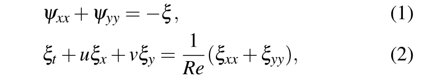
whereuandvare the velocity components in thex- andydirections respectively,Reis the Reynolds number,ψis the stream function andξis the vorticity function, andu=ψy,v=−ψx. Equation (1) is referred to as the stream function equation,equation(2)is referred to as the vorticity equation.
The non-dimensional computational domain is set to{(x,y)|:0≤x ≤1,0≤y ≤1}. The boundary conditions are given as follows:

Because the vorticity on the wall is unknown,in the process of solving Eq.(2),the condition of vorticity on the boundary must be supplemented.In this paper,the numerical boundary conditions of vorticity in Ref.[14]are used,namely,
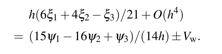
Here, the subscripts 1, 2, 3 represent the boundary point, its neighbor and its sub-neighbor points respectively.Vmis the tangential velocity of the wall. On the sliding wall,Vw=1.On the solid wall,Vw=0.

Fig.1. Schematic of lid–driven square cavity.
At first, an unexpected balance of viscous and pressure forces causes the fluid to turn into the unit square cavity. The properties of these forces depend upon the Reynolds number,and a hierarchy of eddies develops. First, a larger clockwiserotating primary vortex(PV)arises. Its location occurs toward the geometric center of the unit square cavity. Then, several small eddies arise: counterclockwise-rotating secondary eddies, and clockwise-rotating tertiary eddies. Their locations occur at the three relevant corners of the square cavity (bottom right(BR),bottom left(BL),and top left(TL)),appearing hierarchically at the inclined ellipses in Fig.1.
2.2. Numerical method
As the Reynolds number increases, the flow instability starts from the wall boundary layer, where it becomes much thinner under a high Reynolds number. Thus, to predict the third Hopf bifurcation, the boundary layer has to be resolved accurately with either a very fine mesh or high-order numerical method. This makes the numerical simulation very costly and challenging.Eeven worse,recently,it has been found by us[15]that a high-order method might suffer from numerical instability inside the wall boundary layer if a lower-order treatment of boundary conditions is equipped.Such lower-order techniques of wall treatment are very popular in applications of high-order numerical methods. To fix this problem,we have developed a consistent fourth-order compact finite difference scheme,[15]in which both the order of accuracy and the major truncation error term are kept the same for the inner and boundary schemes. Such a high-order scheme can efficiently suppress the numerical instability inside the wall boundary layer. In this work, the numerical method employed is the consistent fourth-order compact finite difference scheme.[15]
After spatial discretization with the consistent fourthorder compact finite difference scheme,an explicit third-order TVD Runge–Kutta scheme[16]is used to perform time discretization.
Mesh convergency for the numerical method is carried out with a driven square cavity withRe= 12500. Table 1 shows the values of velocity at a fixed point(x,y)=(0.5,0.5)of the cavity when the fluid reaches the quasi-periodic state(t=3000) using three uniform meshes (65×65, 129×129,and 257×257)atRe=12500. It can be seen that the results under grid 129×129 are in good agreement with those under the fine grid 257×257 and the maximum error is less than 0.1%.
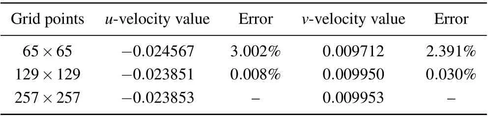
Table 1. Comparison of the values of velocity at a fixed point (x,y) =(0.5,0.5) of the cavity when the fluid reaches the quasi-periodic state at Re=12500.
Based on the mesh convergence test of the above benchmark simulation, in this paper, we take a time step size of∆t=1×10⁻³and solve the system with 129×129 uniform grids in the numerical simulations.
3. Third Hopf bifurcation
3.1. Scenario for the transition to chaos
We determine the different states of the flow according to the time evolution of velocity at a fixed point (x,y) =(0.5,0.5) of the cavity. It is well known that the flow in a lid–driven square cavity becomes quasi-periodic when the Reynolds number is larger than a critical number ofRec2,which is beyond 10000. The flow atRe=12500 is still quasiperiodic in its second Hopf bifurcation as disclosed by Wanget al.[13]

Fig.2. Time history of u-velocity for Re=20000.
We first calculated the flow with a higherRe=20000 fortfrom 0 to 4000 as shown in Figs.2(a)and 3(a)for the evolution ofu-velocity andv-velocity at the geometric center point.
We enlarged Figs.2(a)and 3(a)fortfrom 3960 to 4000 and found that the flow was under chaos as shown in Figs.2(b)and 3(b)for evolution of the respectiveu-andv-velocity components at the geometric center point. From the enlarged figures, one can observe that the flow eventually evolves into a chaotic state.
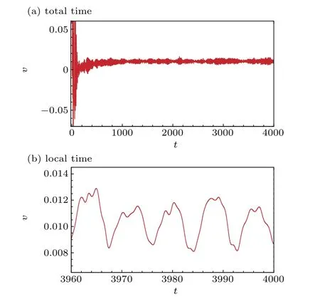
Fig.3. Time history of v-velocity for Re=20000.
3.2. Critical Reynolds number of the third Hopf bifurcation
The above results atRe= 12500 andRe= 20000 imply that the critical Reynolds number ofRec3is located between 12500 and 20000. We began to findRec3by the method of bisection. Starting froma0= 12500,b0= 20000, if atRe=(ak+bk)/2,we get quasi–periodic solution,then we letak=(ak+bk)/2;If atRe=(ak+bk)/2 we get a chaos solution, then we letbk=(ak+bk)/2. We repeated this process and carried out the dichotomy for 12 times,and we got a very small interval. Finally, in this way,Rec3was localized in the small interval (13944.7021,13946.5333). Table 2 shows the process of localizing the range ofRec3by bisection.
In a series of Figs.4 and 5,we present the time history ofu(t)for different Reynolds numbers. In these graphs,we can clearly see that during the process of determining the critical Reynolds number, the functionu(t) solution is either quasiperiodic or chaotic.
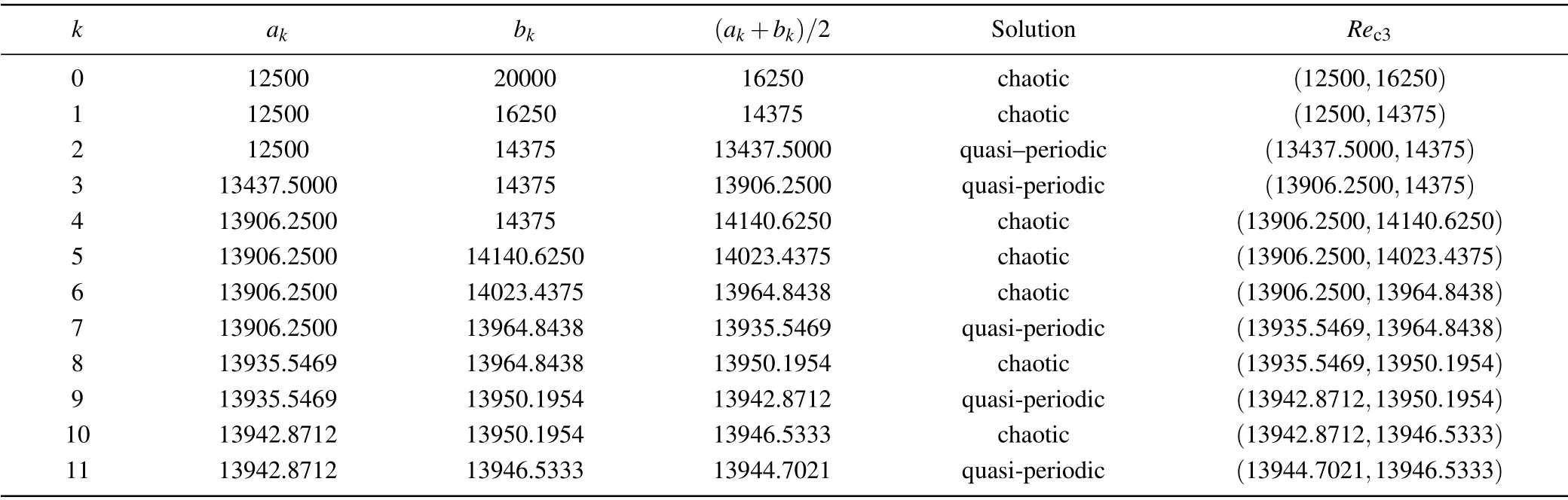
Table 2. Process of bisection for confirming Rec3.

Fig.4. Time history of u-velocity for different Reynolds numbers: (1)total time;(2)local time.

Fig.5. Time history of u-velocity for different Reynolds numbers: (1)total time;(2)local time.

Fig.6. (a1)–(e1)Time history(left figures)of u-velocity from t=3960.0 to t=4000.0;(a2)–(e2)power spectrum density(right figures)of u-velocity for different Reynolds numbers.
3.3. Type of third Hopf bifurcation
The nontrivial succession of periodic,quasi-periodic and eventually seemingly random regimes is reminiscent of the transition to chaos.
It can be seen from Ref.[17]that the route of chaos follows one of the three canonical scenarios: the Ruelle–Takens–Newhouse scenario;[18]the Feigenbaum scenario;[19,20]or the Pomeau–Manneville scenario.[21]The characteristic features of each of these scenarios can be tracked from the evolution of the dominating frequencies of the system.[22]Thus, we shall analyze the main frequencies of velocity fluctuations and seek which classical scenario follows during the flow transition to chaos in the cavity.
We focus on the evolution ofu(t)for different Reynolds numbers fromt=3960 tot=4000 as shown in Figs.6(a1)–(e1). Without loss of generality, we analyze the time series data ofuin Figs. 6(a2)–(e2) via the power spectrum density(PSD).The PSDs(ω)is the square mean of the Fourier transformF(t)of the sample time series,
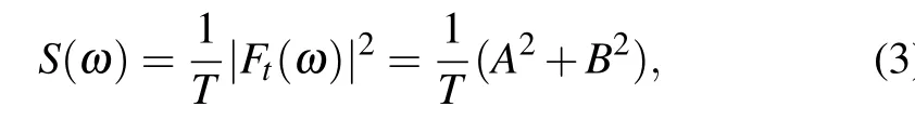
whereAandBare the real and imaginary parts of the complex number,respectively. We usefto express the frequency andf= 1/T. The time series and power spectrum of velocityuare given in Figs. 6(a2)–6(e2). In these figures, the left figures shows the time series ofuat different Reynolds numbers,and their corresponding PSDs are shown in the right figures. AtRe= 10000 as shown in Fig. 6(a2), there is only a frequency indicating the flow is periodic. When the Reynolds number increases,we can see that the flow tends to be quasi-periodic with two frequencies atRe=12500. The flow becomes chaotic with four frequencies asReincreases toRe=15000 from Fig. 6(c2). The number of frequencies increases to six whenRe=17500 as observed in Fig. 6(d2).Further, asReincreases toRe=20000, the number of frequences increases to eight with two primary frequencies and six secondary frequencies found from Fig. 6(e2). The series of PSD figures shows no existence of odd number frequencies and exhibits a characteristic of period-doubling bifurcation.
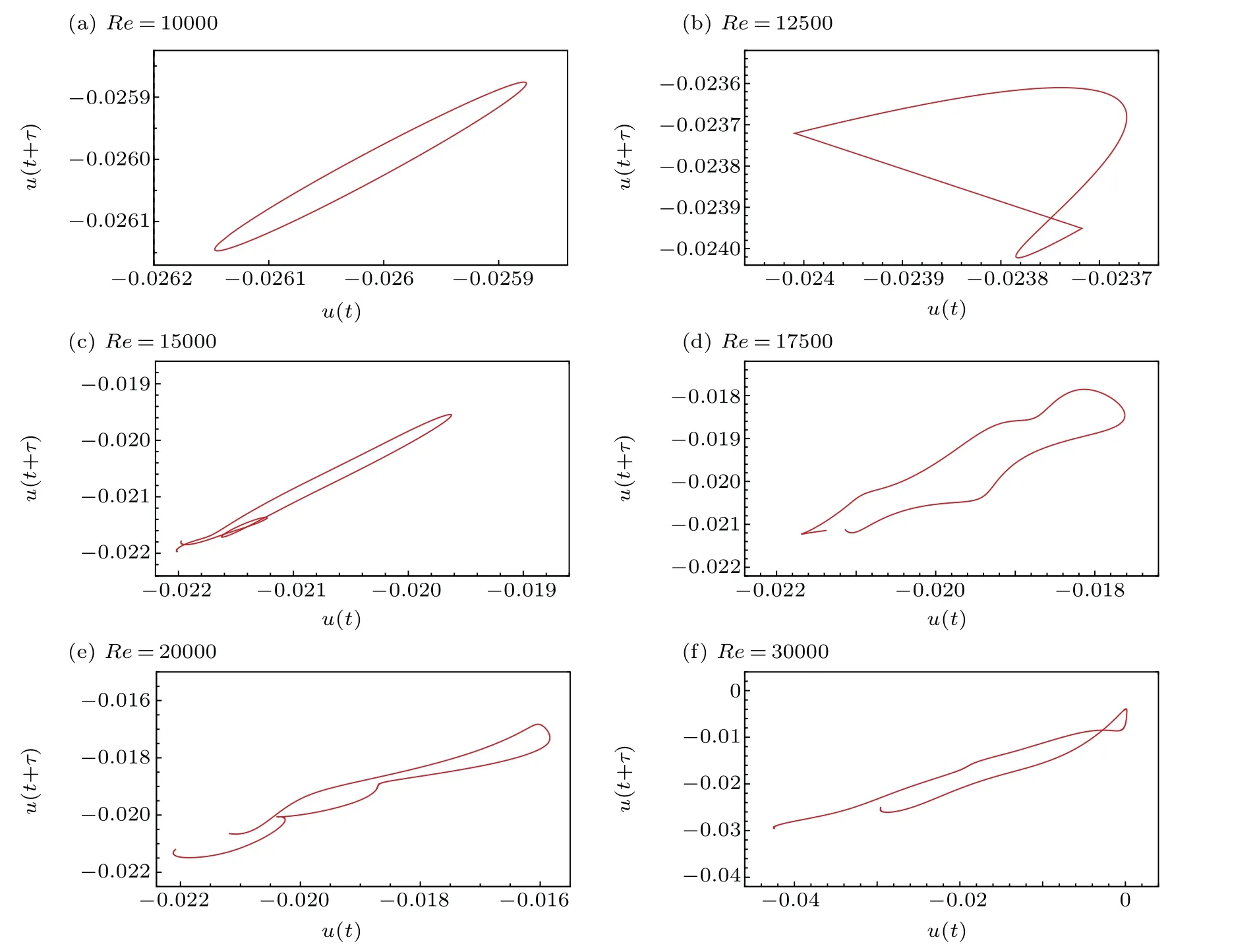
Fig.7. Phase portrait of u(t)for different Reynolds numbers.
4. Characterization of the dynamical system
Theoretically,a chaotic dynamical system cannot be fully characterized by means of frequency spectra. In particular,spectra do not offer a way to distinguish a stochastic system from a chaotic one. To ascertain the possible chaotic nature of the flow system in the cavity,most scholars seek to characterize the underlying dynamics by means of nonlinear time series analyses of the attractor,[23]Kolmogorov entropy[24]and maximal Lyapunov exponent.[25,26]In this paper,we also ascertain it by these means.
4.1. Attractor
We reconstruct the two-dimensional phase space of the time series ofu(t) fromt= 3960 tot= 3964 at different Reynolds numbers.
Packard[27]proposed to reconstruct the phase space equivalent to the original phase space of the system by restoring the attractor of the dynamical system from scalar time series. The time delay method is to reconstruct the phase space by selecting the appropriate time delay and embedding dimension for the one-dimensional time series and further observe the attractor characteristics of the phase space. According to embedding theory,[28]it can be reconstructed by selecting the appropriate reconstruction dimensionmand delay timeτfor the one-dimensional time series and anm-dimensional phase space can be reconstructed. In this paper,we rearrange the original time series into a two-dimensional distribution(m=2),namely,

The autocorrelation method[29]is used to calculate the time delayτ.We calculate the time delayτ= 1.818,1.429,7.500,7.500,8.000,9.2000 forRe=10000,12500,15000,17500,20000,30000.
Then,we can draw a two-dimensional phase distribution to study the evolution of its phase diagram and attractor of the system with Eq. (4). Figures 7(a)–(f) show the evolution of the phase diagram and thus the characteristics of the attractor at various Reynolds numbers. The series of phase diagrams shows a change from an ellipse closed form at the periodic state to a non-ellipse closed form at the quasi-periodic state and finally to an unclosed curve. The attractor of the system changes from the normal to a strange one. This implies that the flow system eventually becomes chaotic whenRe ∈[Rec3,30000].
4.2. Kolmogorov entropy
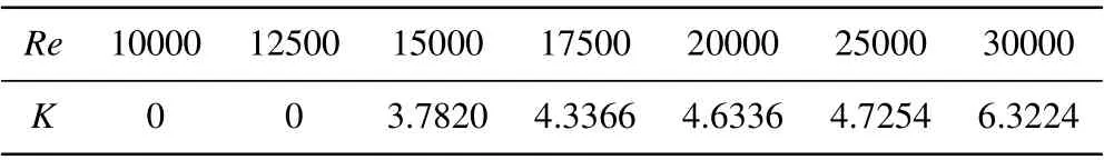
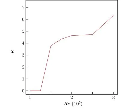
We compute the Kolmogorov entropy(denoted byK)of the time series ofu(t) fromt=0 tot=4000 for different Reynolds numbers.
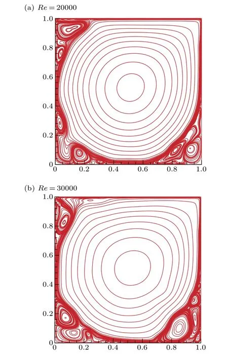
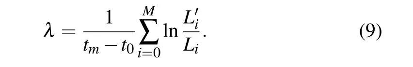
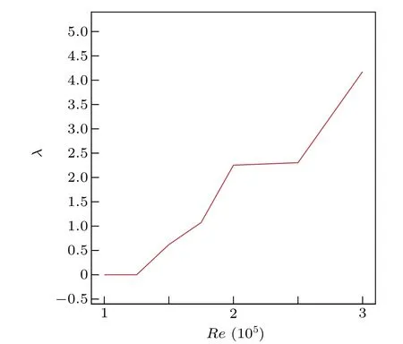
The Kolmogorov entropy can be computed by the method proposed in Ref. [30]. Theoretically, a chaotic (deterministic) system is characterized with a positive finite value of 0 At present, the correlation integralC2(m,ε) is widely used in the literature to calculateK,called the correlation entropy. The specific calculation process is as follows: (i) For the time seriesu(t), we reconstruct the phase spaceU(t) according to form Eq.(4);two of the vectors areUi(i.e.i=1,2).(ii)The Euclidean distance from the remainingn−1 points toUiis calculated by selecting any point from thenpoints inUi K2entropy is usually used as an approximation ofK. Table 3 shows the value ofKis zero forReequal to 10000 or 12500. Thus the system is in order. This is consistent with the conclusion of Ref.[13].The value ofKis greater than zero for 15000≤Re ≤20000.Thus the system is in chaos.We continue to calculate theKvalue forRe=25000,30000;the value ofKincreases with increasing Reynolds number. As a result,the flow system in the cavity is chaotic forRe ∈[Rec3,30000]. Table 3. Kolmogorov entropy for different Reynolds numbers. Figure 8 shows the variation of theKvalue for different Reynolds numbers. It shows that asReincreases,the value ofKincreases. Fig.8. Variation of K value for different Reynolds numbers. In order to observe the subtle changes of the whole flow field more clearly,without loss of generality,we give the twodimensional stream function contours for different Reynolds numbers. Figure 9 shows the contours of the stream function forRe=20000,30000. It can be seen from Fig. 9 that the streamlines in the middle of the cavity are smooth while in three corners of the cavity they are twisted. This is why the values ofKare not as large. Fig.9. Streamlines for different Reynolds numbers. The chaotic behavior atRe ∈[Rec3,30000]can be characterized further by computing the maximal Lyapunov exponent(denoted byλ).λis computed as the rate of spatial divergence in the phase space of two trajectories that are initially in the same neighborhood.[31]In a deterministic system,the existence of dynamic chaos can be intuitively judged from whether the maximum Lyapunov exponent is greater than zero. If the maximum Lyapunov exponent of the system is positive(λ> 0), the system is chaotic; the higher the value is, the more chaotic the system is. Otherwise, the system is ordered(λ ≤0). Here, we apply the Wolf method[32]to computeλof the time series ofu(t) fromt= 0.0 tot= 4000.0 for different Reynolds numbers. The specific calculation process is as follows: For the time seriesu(t), we (i)reconstruct the phase spaceU(t) according to form Eq. (4), (ii) take the initial pointU0(t0) and find the nearest neighbor of the initial pointU0(t0), let it beU(t0) and then let the Euclidean distance between the two points beL0, (iii) track the evolution trajectory ofU0(t0)andU(t0)with time untilt1,when the distance between them exceeds a certain specified valueε>0 :ifL′0=|U(t1)−U0(t1)|>εthen keepU(t1)and find another pointU1(t1),such thatL1=|U(t1)−U1(t1)|<εand the angle between them is as small as possible, (iv)continue the above process untilU(t) reaches the end pointN(Nis the length of the time series). Let the total number of iterations in the evolution process beM;then the formula forλis We obtainλfor different Reynolds numbers. The results are shown in Table 4. Table 4 shows the value ofλis 0 forReequals to 10000 or 12500. Thus the system is in order. This is again consistent with the conclusion of Ref.[13].The value ofλis greater than 0 for 15000≤Re ≤20000, which confirms the chaotic behavior of the system. We continue calculate theλvalue forRe=25000,30000 and findλ>0. As shown in Fig. 10, one can see the variation ofλvalue for different Reynolds numbers. The value ofλincreases asReincreases. In conclusion,the various nonlinear analyses above confirm the presence of chaos forRe ∈[Rec3,30000]. Table 4. Maximal Lyapunov exponent for different Reynolds numbers. Fig.10. Variation of λ value for different Reynolds numbers. In this paper, we presented a numerical investigation on the pathway to chaos in driven square cavity flow.The flow dynamics were analyzed by means of the time series of theu-velocity component obtained by direct numerical simulation of the unsteady two-dimensional Navier–Stokes equations.As a first result,we confirmed the existence of the third Hopf bifurcation as the Reynolds number increases and located the critical Reynolds number of the third Hopf bifurcation(Rec3)in the interval of(13944.7021,13946.5333). Moreover, by analyzing the time series of theu-velocity component, we disclosed that its successive bifurcation is period-doubling and the flow becomes chaotic when the Reynolds number is beyondRec3. The chaotic characteristics were further confirmed via analysis of the Kolmogorov entropy,maximum Lyapunov exponent and phase diagram. Acknowledgment The authors thank Professor Yong Xu of the Northwestern Polytechnical University for helpful discussion.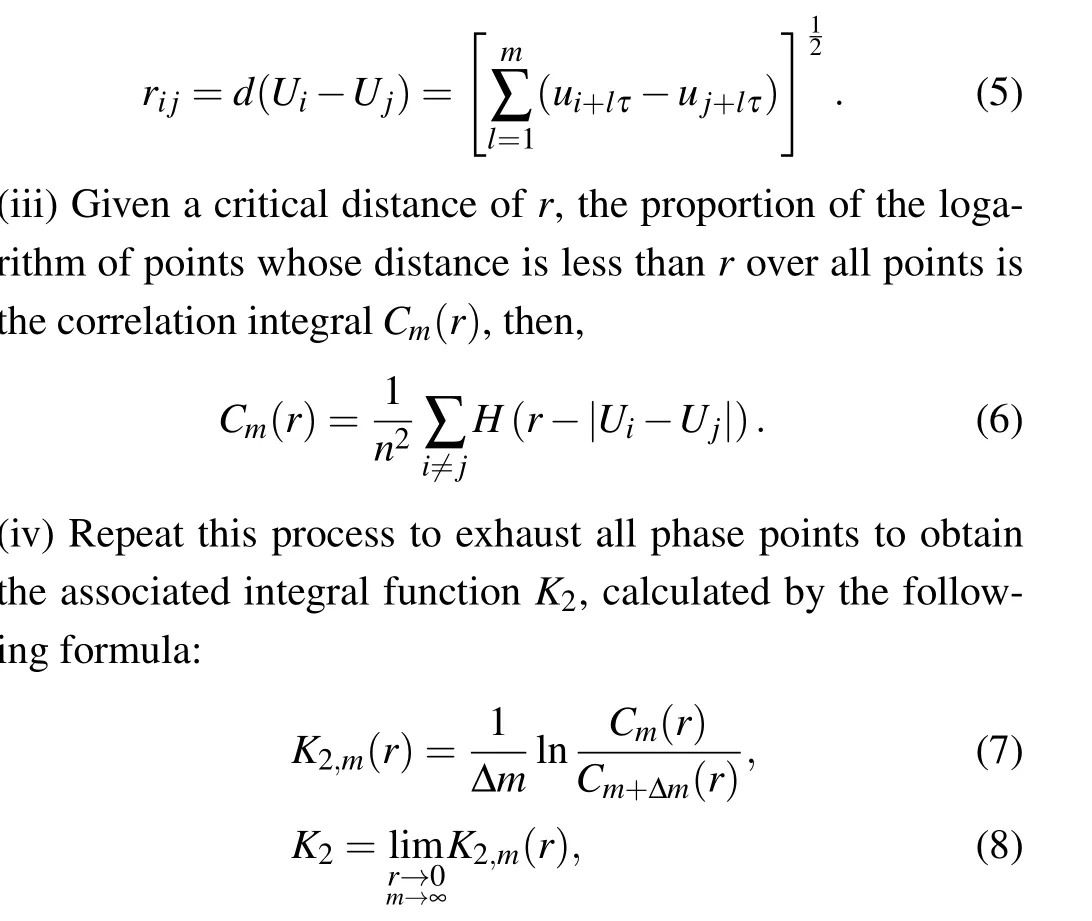
4.3. Maximal Lyapunov exponent

5. Conclusion
猜你喜欢
Chinese Physics B(2023年1期)2023-02-20
理科爱好者(教育教学版)(2022年2期)2022-05-05
Plasma Science and Technology(2022年2期)2022-03-10
大众文艺(2020年23期)2021-01-04
大众文艺(2020年22期)2020-12-13
艺术家(2018年12期)2018-03-18
水动力学研究与进展 B辑(2017年1期)2017-03-09

- Chinese Physics B的其它文章
- Transient transition behaviors of fractional-order simplest chaotic circuit with bi-stable locally-active memristor and its ARM-based implementation
- Modeling and dynamics of double Hindmarsh–Rose neuron with memristor-based magnetic coupling and time delay∗
- Cascade discrete memristive maps for enhancing chaos∗
- A review on the design of ternary logic circuits∗
- Extended phase diagram of La1−xCaxMnO3 by interfacial engineering∗
- A double quantum dot defined by top gates in a single crystalline InSb nanosheet∗