The U.S.Experience with Developing and Implementing a Probability Based Limit States Bridge Specification

J.M.Kulicki

(Modjeski＆ Masters，Inc.，Mechanicsburg，Pennsylvania，USA)

1 The Past-Historical Development(1986－1993)

1.1 Background

The apparent start of the process leading to implementation of load and resistance factor design(LRFD)in the AASHTO LRFD Bridge Design Specifications［3］was the initiation of The National Cooperative Highway Research Program(NCHRP)Project 20-7/31，entitled“Development of Comprehensive Bridge Specification and Commentary”(1987)，in August of 1986.In reality，the process leading to this decision had started decades earlier.Engineers in Europe had an early start on consideration of limit states design and reliability-based design.Their pioneering efforts provided a history of successful experience which validated the underlying concepts.In 1979，the first edition of the Ontario Highway Bridge Design Code(OHBDC)(Ontario Ministry of Transportation 1991)was released to the design community as North America’s first calibrated，reliabilitybased limit states bridge specification.Since that time，the OHBDC has been updated in 1983 and 1992 and rereleased.Very significantly，the code contained a companion volume of commentary.It has now been replaced by the Canadian Highway Bridge Design Code.

U.S.engineers recognized a certain logic in the calibrated limit states design and began to question whether the AASHTO Standard Specification for Highway Bridges(StandardSpecifications)(AASHTO 2002)should be based on a comparable philosophy for determining the safety of structures.Many research projects，undertaken by the NCHRP，the National Science Foundation(NSF)，and various states were bringing new information on bridge design faster than it could be critically reviewed and，where appropriate，adopted into the Standard Specification.It was also becoming clear that the many revisions which had occurred to the Standard Specification had resulted in numerous inconsistencies and the appearance of a“patchwork”document，a term coined by some of the State Bridge Engineers.

In the spring of 1986，a group of State Bridge Engineers or their representatives met in Denver，Colorado，and drafted a letter to the Subcommittee on Bridges and Structures(SCOBS)indicating their concern that the Standard Specification was falling behind the times.They also raised the concern that the Technical Committee structure，operating under the SCOBS was not able to keep up with emerging technologies.Presentations were made at two regional meetings to mixed reception.Nonetheless， this group planted the seed which led to the development of the AASHTO LRFD.

In July of 1986，a different group of State Bridge Engineers met with the staff of the NCHRP to consider whether a project could be developed to explore the points raised in the Denver letter.This led to NCHRP Project20-7/31“DevelopmentofComprehensive Bridge Specifications and Commentary”，a pilot study conducted by Modjeski and Masters，Inc.with the following Scope:

Task 1－Review of the philosophy of safety and coverage provided by other specifications.

Task 2－Review the Standard Specifications for content and review other AASHTO documents for their potential for inclusion into a Standard Specification.

Task 3－Assess the feasibility of a probabilitybased specification.

Task 4－Prepare an outline for a revised AASHTO specification for highway bridge design，and a commentary，and present a proposed organizational process for completing such a document.

The Task 1 review of other specifications and the trends in the development of new specifications included a review of work done in Canada(especially the Province of Ontario)，Great Britain，the Federal Republic of Germany and Japan.Personal contacts with practitioners and researchers in other countries provided information on the emerging directions of specification development and insight into what designers were doing to implement specifications，and，in some cases，what designers were choosing not to implement based on a perception of unnecessary complication.Information collected from these various sources indicated that most of the industrialized countries appeared to be moving in the direction of a calibrated，reliability-based，limit states specification.

Task 2 can best be summarized as a search for gaps and inconsistencies in the 13th Edition of the Standard Specifications.“Gaps”were areas where coverage was missing;“inconsistencies”were internal conflicts，or contradictions of wording or philosophy.Many gaps and inconsistencies were found and they are summarized elsewhere［24］.

With respect to Task 3 and the feasibility of using probability-based limit states design，a review of the philosophy used in a variety of specifications resulted in three possibilities，two of which are already included in the then current specification.They are:

Allowable stress design(ASD)which treats each load on the structure as equal from the view point of statistical variability.A“common sense”approach may be taken to recognize that some combinations of loading are less likely to occur than others，and a higher working stress may be allowed for these load combinations.

Load Factor Design(LFD)-In which a preliminary effort was made to recognize that the live load，in particular，was more highly variable than the dead load.This thought is embodied in the concept of using a different multiplier on dead and live load，e.g.，a load combination involving 130%of the dead load combined with the 217%of the live load，and requiring that a measure of resistance based primarily on the estimated peak resistance of a cross-section exceed the combined load.

Reliability-based design which seeks to take into account directly the statistical mean resistance，the statistical mean loads，the nominal，or notional，value of resistance，the nominal or notional value of the loads and the dispersion of resistance and loads as measured by either the standard deviation or the coefficient of variation，i.e.，the standard deviation divided by the mean.This process can be used directly to compute the relative probability of failure for a given set of loads，statistical data and the Designer’s estimate of the nominal resistance of the component being designed.Thus，it is pos-sible to vary the nominal resistance to achieve a criteria which might be expressed in terms such as the component(or system)must have a probability of failure of less than 0.0001，or whatever value is acceptable to society.Alternatively，the process can be used to target a quantity known as the“reliability index”which is somewhat，but not directly，relatable to the probability of failure.Based on this“reliability index”，it is possible to reverse engineer a combination of load and resistance factors to achieve a specific reliability index.

While some specifications were being developed in terms of the“probability of failure”，it was generally agreed that it would be more appropriate to use the reliability index process to develop load and resistance factors.That way，design could proceed in a process directly analogous to Load Factor Design as it appeared in the then current 13th Edition of the Standard Specification.

The discussion of the three possible philosophical bases for specifications can be put in equation form expressing structural sufficiency.This is shown in Equations 1 through 3 for ASD，LFD，and LRFD，respectively.

where，Qi=a load;RE=elastic resistance;FS=factory of safety.

where，γi=a load factor;Qi=a load;R=resistance;φ=a strength reduction factor.

where，ηi= ηDηRηI≥0.95 for loads for which a maximum value of γiis appropriate，and ηi=1/ηIηDηR≤1.0 for loads for which a minimum value of γiis appropriate;ηi=load factor:a statistically based multiplier on force effects;φ=resistance factor:a statistically based multiplier applied to nominal resistance;ηi=load modifier;ηD=a factor relating to ductility;ηR=a factor relating to redundancy;ηI=a factor relating to operational importance;Qi=nominal force effect:a deformation，stress，or stress resultant;Rn=nominal resistance:based on the dimensions as shown on the plans and on permissible stresses，deformations，or specified strength of materials;Rr=factored resistance:φRn.

In May of 1987，the findings of NCHRP Project 20-7/31 were presented to the AASHTO SCOBS outlining the information above and indicating that seven options appeared to be available for consideration［24］.The Subcommittee requested funding through the AASHTO Standing Committee on Research for the NCHRP to initiate a project to develop a new，modern bridge design specification.This led to NCHRP Project 12-33 which was also entitled“Development of Comprehensive Specification and Commentary”［22］.Modjeski and Masters，Inc.began work in July，1988.

1.2 Development Objectives

There were several objectives in the development of this new specification.They may be summarized as:

1)To develop a technically state-of-the-art specification which would put U.S.practice at or near the leading edge of bridge design.

2)To make the specification as comprehensive as possible and include new developments in structural forms，methods of analysis and models of resistance.

3)To the extent consistent with the thoughts above，keep the specification readable and easy to use，bearing in mind that there is a broad spectrum of people and organizations involved in bridge designs.

4)To keep specification-type wording and not to develop a textbook.

5)To encourage a multi-disciplinary approach to bridge design，particularly in the area of hydraulics and scour，foundation design and bridge siting.

6)To place increasing importance on the redundancy and ductility of structures.

To achieve the objectives above，the new specifications had to be markedly different from the Standard Specifications.Many changes had to be made in both the content and appearance.Areas of major changes are identified below:

1)The introduction of a new philosophy of safety-LRFD.

2)The identification of four limit states.

3)The development of new load factors.

4)The development of new resistance factors.

5)The relationship of the chosen reliability level，the load and resistance factors，and load models through the process of calibration.

6)The development of improved load models necessary to achieve adequate calibration，including a new live load model.

7)Revised techniques for analysis and the calculation of load distribution.

8)A combined presentation of plain，reinforced，and prestressed concrete.

9)The introduction of limit state-based provisions for foundation design and soil mechanics.

10)Expanded coverage on hydraulics and scour.

11)Changes to the earthquake provisions to eliminate the seismic performance category concept by making the method of analysis a function of the importance of the structure.

12)Guidance on the design of segmental concrete bridges.

13)Inclusion of large portions of the FHWA Specification for ship collision.

14)Expanded coverage on bridge rails based on crash testing，with the inclusion of methods of analysis for designing the crash specimen.

15)The introduction of the isotropic deck design process.

16)The development of a parallel commentary.

1.2.1 Introduction to Reliability as a Basis of Design Philosophy

1)An introduction to probability-based reliability theory can be simplified considerably by initially considering that natural phenomena can be represented mathematically as normal random variables，as indicated by the well-known bell-shaped curve.This assumption leads to closed form solutions for areas under parts of this curve，as given in many mathematical handbooks and programmed into many hand calculators and spreadsheets.

2)Accepting the notion that both load and resistance are normal random variables，the bell-shaped curve corresponding to each of them can be plotted in a combined presentation dealing with distribution as the vertical axis against the value of load，Q，or resistance，R，as shown in Fig.1.The mean value of loadand the mean value of resistance()are also shown.For both the load and the resistance，a second value somewhat offset from the mean value，which is the"nominal"value，or the number that designers calculate as the load or the resistance is also shown.The ratio of the mean value divided by the nominal value is called the"bias".The objective of a design philosophy based on reliability theory，or probability theory，is to separate the distribution of resistance from the distribution of load，such that the zone where load is greater than resistance is tolerably small.In the particular case of the LRFD formulation of a probability-based specification，load factors，and resistance factors are developed together in a way that forces the relationship between the resistance and load to be such that the zone is less than or equal to the value that a code-writing body accepts.Note in Fig.1 that it is the nominal load and the nominal resistance，not the mean values，which are factored.A conceptual distribution of the difference between resistance and loads，combining the individual curves discussed above，is shown in Fig.2.

Fig.1 Separation of loads and resistance图1 荷载与阻力的分离

Fig.2 Reliability indices inherent in ASHTO LRFD图2 ASHTO LRFD规范采用的可靠指标

It now becomes convenient to define the mean value of resistance minus load as some number of standard deviations，βσ，from the origin.The variable"β"is called the"reliability index"and"σ"is the standard deviation of the quantity R－Q.The problem with this presentation is that the variation of the quantity R－Q is not explicitly known.Much is already known about the variation of loads by themselves or resistances by themselves，but the difference between these had not yet been quantified.However，from the probability theory，it is known that if load and resistance are both normal and random variables，then the standard deviation of the difference is:

Given the standard deviation and considering Fig.2 and the mathematical rule that the mean of the sum or difference of normal random variables is the sum or difference of their individual means，we can now define the reliability index，β，as:

Comparable closed-form equations can also be established for other distributions of data，e.g.，log-normal distribution.A"trial and error"process is used for solving for β when the variable in question does not fit one of the already existing closed-form solutions.

The process of calibrating load and resistance factors starts with Equation(5)and the basic design relationship;the factored resistance must be greater than or equal to the sum of the factored loads:

Solving for the average value of resistance yields:

Using the definition of bias，indicated by the symbol λ，Equation(6)，leads to the second equality in E-quation(7).A straightforward solution for the resistance factor，φ is:

Calibration was done using a suite of test bridge designs.A simulated set of 91 bridges based on 175 real bridges was developed which was comprised of:

1)Twenty-five non-composite steel girder bridge simulations for bending moments and shear with spans of 9，18，27，36 and 60 m，and for each of those spans，spacings of 1.2，1.8，2.4，3.0 and 3.6 m.

2)Representative composite steel girder bridges for bending moments and shear having the same parameters as those identified above.

3)Representativereinforced concreteT-beam bridges for bending moments and shear having spans of 9，18，27 and 39 m，with spacings of 1.2，1.8，2.4 and 3.6 m in each span group.

4)Representative prestressed concrete I-beam bridges for moments and shear having the same span and spacing parameters as those used for the steel bridges.

Full tabulations of these bridges and their representative amounts of the various loads are presented in Nowak［25］.

The reliability indices were calculated for each simulated bridge for both shear and moment.The range of reliability indices which resulted from this phase of the calibration process is presented for the 91 simulated bridges in Fig.3 from Kulicki，et al［18］.It can be seen that a wide-range of values were obtained using the current specifications，but this was anticipated based on previous calibration work done for the OHBDC［28］.

Fig.3 Definition of reliability index，β图3 可靠指标β的意义

Reliability indices were recalculated for each of the 91 simulated cases using the new load and resistance factors.The results are shown in Fig.4.

Fig.4 Reliability indices inherent in the 13th Edition of the Standard Specifications图4 第13版标准规范采用的可靠指标

Fig.4 shows that the new calibrated load and resistance factors，and new load models and load distribution techniques work together to produce very narrowly-clustered reliability indices close to the selected target of 3.5.This was the objective of developing the new factors.Correspondence to a reliability index of 3.5 is something which can now be altered by AASHTO.The target reliability index could be raised or lowered as may be advisable in the future and the factors can be recalculated accordingly.This ability to adjust the design parameters in a coordinated manner is one of the strengths of a probabilistically-based reliability design.

1.2.2 Reassessment of the Original LRFD Calibration

The reliability analysis procedure applied in the original calibration of AASHTO LRFD was based on a simplified calibration procedure based on Rackwitz and Fiessler procedure［26、29］. The Rackwitz and Fiessler method is based on approximation of non-normal random variables by normal variables that satisfy special requirements.The approximating normal variables must have the same value of the cumulative distribution function(CDF)and probability density function(PDF)as the original(non-normal)variable at the so called“design point”.Using the Rackwitz and Fiessler procedure，the reliability index and“design point”are determined by iterations.Loads were assumed to be normal and resistance lognormal.The lognormal distribution for resistance has to be approximated using a normal distribution at the“design point”.Based on experience from extensive reliability analysis，it was found that for structural components the“design point”is equal to about 2 standard deviations from the mean.This observation allowed for derivation of a closed-form formula for the reliability index that has been used in bridge calibration with success［26］. However， other methods are now widely used which eliminate the need to approximate the lognormal distribution.

Currently the most efficient and accurate method for calibration is based on Monte Carlo simulations.In the past，the application of Monte Carlo technique was limited by the availability of fast computers.This is not a problem anymore and，therefore，Monte Carlo is a leading contender for future calibration work.

The typical application of Monte Carlo simulation for bridge-structures reliability as reported in the literature［11，27］is as follows:

1)Load is usually assumed to be normally distributed.The load side of the LRFD equation is a summation of force effects and thus has been assumed to be normally distributed.

2)Resistance is usually assumed to be lognormally distributed.The resistance side of the LRFD equation is a product of terms and thus has been assumed to be lognormally distributed.

Using the reported statistics of load and resistance and computer-generated random numbers，the distributions of load and resistance are basically reconstituted and values chosen randomly from these reconstituted distributions.For example for the simple load combination of dead load plus live load，random values of dead load and live load are chosen from the reconstituted normal distributions of dead and live load respectively.A random value of resistance is chosen from the reconstituted lognormal distribution of resistance.

The limit-state function，Ri-(Di+Li)is calculated.If the value is equal to or greater than zero，the function is satisfied and the individual case is safe.If the value is negative，the criterion is not satisfied and it fails.

After a number of iterations，the failures are counted and the failure rate determined.For the sampling to be significant at least ten failures should be observed，otherwise，more iteration is necessary.

Using the failure rate，the reliability index is determined as the inverse of the standard normal cumulative distribution.

Several observations can be made regarding this process:

The solution is only as good as the modeling of the distribution of load and resistance.

If load is not correctly modeled as normally distributed or resistance is not correctly modeled as lognormally distributed，the solution is not accurate.Further，if the statistical parameters(in other words，mean，standard deviation and bias)are not well defined，the solution is equally inaccurate.

If both the distribution of load and resistance are normally or lognormally distributed then the closed-form formulas provide accurate results.If this is not the case，then Monte Carlo simulation can produce accurate solutions.The accuracy depends on the number of simulations.

The power of the Monte Carlo simulation is its ability to use a variety of distributions for load and resistance.

A study was made for project NCHRP 20-7/186 as reported in Kulicki et al［19］comparing the results of a million iterations of the Monte Carlo simulation to the results of the Rackwitz and Fiessler procedure embodied in spreadsheets used in the original calibration of the LRFD Specification.The sole purpose of this analysis was to verify that the Monte Carlo and Rackwitz and Fiessler methods would give sufficiently similar results for the cases studied.Fig.5 shows the result of that analysis for each of the structures identified above for bending moment.A perfect comparison between the two methods would be indicated by a 100%value on Fig.5.Each of the dots are actually values for each of the spacings identified above.Thus in the top panel of Fig.5，the left most dot is actually five data points that are so close together that the difference cannot be discerned in the plot.The small differences that do exist can be attributed in part to the slight difference in the statistical parameters used between the two methods.In the implementation of the Rackwitz-Fiessler procedure，Nowak differentiated between the dead load due to factory-built and field-built components with slightly different values of bias and coefficients of variation.The Monte Carlo simulations presented herein combined these two load components and used“average”values for the bias and coefficient of variation.Fig.5 indicates that the results are in sufficient agreement.

As part of the work in NCHRP 20-7/186，the Monte Carlo method of simulation as described above was applied to 124 additional bridges.Fig.6 shows the beta factors for the entire set of bridges in the database.In general，the range of results is similar to that obtained in the original calibration report［26］.

Fig.5 Comparison of the results of the Monte Carlo Simulation and Rackwitz and Fiessler method图5 Monte Carlo模拟法、Rackwitz和Fiessler 3种方法计算结果比较

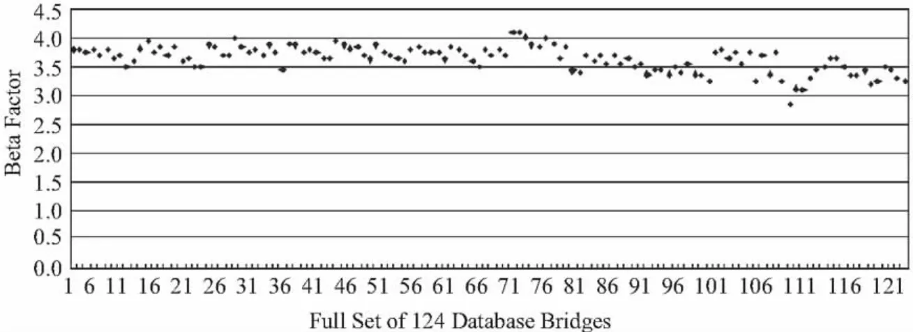
Fig.6 Monte Carlo results for all bridges in the database图6 使用Monte Carlo法计算各桥梁的结果

1.2.3 Rationale for a New Live Load Model

Early editions of the AASHTO Standard Specification contained a representation of a truck and/or a group of trucks for use in design.The very earliest editions of this Specification contained a single unit truck weighing up to 178 kN(20 U.S.customary tons)，which was known as the H20 truck.Lighter variations of this vehicle were also considered and were designated as HXX，e.g.，H15.Groups of 133 kN trucks，with an occasional 178 kN truck，were also utilized as a truck-train.

In 1931，the first edition of the Standard Specification instituted the"lane load"，which consisted of a uniform load of 9.3 N per mm and a moving concentrated load or loads.A concentrated load of 116 kN was used for shear and for reaction，two 80 kN concentrated loads were used for negative moment at a support and were positioned in two adjacent spans，and a single 80 kN load was used for all other moment calculations.

In 1944，the design truck was extended into a tractor-semi-trailer combination，known as the H20-S16-44，commonly referred to as simply the HS-20 truck.This vehicle，shown in Fig.7，weighed a total of 325 kN and was comprised of a single steering axle weighing 35 kN and two axles that supported the semi-trailer，each weighing 145 kN.The axles on the semi-trailer could vary from 4.3 m to 9.0 m，and it was assumed that there was 4.3 m between the steering axle and the adjacent axle that formed part of the tractor.The HS-20 truck was an idealization and did not represent one particular truck，although it was clearly indicative of the group of vehicles commonly known as 3 －S2’s，e.g.，the common"18 wheeler".

Fig.7 Configuration of HS-20 truck图7 HS-20货车布置

During the late 1970s and early 1980s，some states raised their design load to HS-25，or 125%of the HS-20 truck and/or the Lane Load.During the construction of the Interstate Highway System，an additional design load，known as the"Interstate Load"，or design tandem was also introduced，and this consisted of two 110 kN axles separated by 1.2 m.Some of the states which raised the design load to HS-25 also increased the weight of the design tandem to 133 kN.

The actual configurations of trucks are almost limitless，and it has long been recognized that the regulatory control of vehicles is a significantly different matter than the choice of a design model upon which to base calculations.The link between these two needs are state legal loads and the Federal Bridge Formula.These two regulatory devices have the objective of recognizing that the commercial needs of the Country can only be satisfied by a plethora of vehicle configurations and that it is sometimes necessary that these configurations create significantly larger force effects in structures than those calculated using the design model.The AASHTO Manual for Maintenance Inspection of Bridges has long recognized this by prescribing two stress levels commonly referred to as the Inventory Level，which approximates design stresses or design force effects and the Operating Level，which results in approximately 1/3 more total force effect on the basis that it will occur，although relatively infrequently.

Over the years，many states have written exclusions into their regulatory policies，which permitted some vehicles in excess of legal loads to operate in an unrestricted manner.These loads are sometimes referred to as"grandfather provision"loads.

As a result of the evolution summarized above，it became increasingly apparent that the HS loading did not bear a uniform relationship to many of the vehicles allowed on the roads.It was becoming out-of-date.In developing a new design specification，it became apparent quite early in the process that if the objective was a more uniform and consistent safety of bridges，a new live load model would be necessary in order to produce that consistency.

In 1990，the Transportation Research Board published Special Report 225，summarizing a study into the state legal loads，grandfather provisions，the current Federal Bridge Formula and various attempts to extend the Federal Bridge Formula，or to develop other regulatory models.This study contained extensive information on the estimated benefits from more efficient movement of goods compared to the cost and accelerated damage to roadways and bridges.A group of vehicles were identified in Special Report 225 and were made available to the LRFD development group as part of personal correspondence.Various vehicle configurations arising from this work are shown in Fig.8.

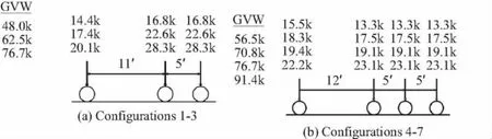
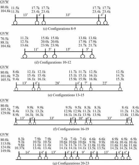
Fig.8 A selection of truck configuration(Note Customary US Units)图8 货车布置选择

The force effect on bridge structures from these various"families"of vehicles were studied by calculating the envelope of force effects from each of the representative vehicles in a"family"for:

1)Centerline moment of a simply-supported girder

2)Positive and negative moment at the 0.4L point of a two-span continuous girder

3)Negative moment at the interior pier of a twospan continuous girder

4)Positive and negative end shear and negative shear at the interior support of a two-span continuous girder

Fig.9 shows a comparison of the various momenttype force effects，identified above，for spans from 6 to 45 m generated by the exclusion vehicles compared to the HS-20 truck.This comparison is developed by plotting the ratio of the force effect from the envelope of exclusion vehicles divided by the corresponding force effect from the HS-20 vehicle on a vertical axis，against span length on the horizontal axis.Thus，a complete match of force effects，indicating that the HS-20 vehicle was an accurate and representative model of the exclusion loads，would be indicated by a horizontal line passing through the vertical axis at a value of 1.0.Corresponding information for the shear force effects identified above are also shown in Fig.9 in which Vab is the shear at the simply-supported end and Vba is the shear adjacent to the interior support.Fig.9 showed that the HS-20 vehicle is not representative of current loads on the highways.

Fig.9 Moments and shears from exclusion vehicles normalized to HS-20图9 除规定车辆HS20外的荷载产生的弯距和剪力

A notional design load，known as the HL93 loading，was chosen after consideration of five possibilities which included an equivalent uniform load，a single multi-axle vehicle，a family of three axle strings and an associated before and after uniform load，HSXX，and the HL93 loading consisting of a combination of either a pair of 110 kN tandem axles and the uniform load，or the HS-20 and the uniform load The HL93 had the best fit to the exclusion vehicles as indicated in Fig.10 which was developed in a manner similar to that in Fig.9，except that results are normalized to the HL93 loading.It also had the virtue of being composed of elements，i.e.，the truck，the lane load，and the tandem axle，which are well-known to designers，albeit applied somewhat differently.

Fig.10 Moments and shears from exclusion vehicles normalized to HL93图10 除规定车辆HSL93外的荷载产生的弯矩和剪力

1.2.4 Rationale for New Live Load Distribution Factors

One of the simplifications that has existed in the AASHTO Specifications，virtually from its beginnings，was an attempt to produce a simple way of determining the amount of live load carried by one element of a bridge system，e.g.，one longitudinal girder.This gives rise to a so called distribution factor which is commonly written as“S/D”where S is the spacing between longitudinal elements and D is a constant.The most common version of this in U.S.units is S/5.5.Early in the Interstate era，when girder spans were relatively short and the elements were relatively close together，this simple expression yielded reasonably realistic results.However，as longer girders replaced truss spans out to about 150 m，and the girder spacing changed from around 2.5 m to 3.5 m to 4.5 m，the simple S/D expression became increasingly more unrealistic.Fortunately，the results obtained with this simple approximation were usually quite conservative.This has been verified through dozens of field stress measurements，as well as analytic investigations going back 40 years or more.The literature is full of countless research efforts oriented towards developing a better approximation.In the design environment，the introduction of matrix structural analysis and，eventually finite element analysis，made it practical for designers to make grid or continuum models of many types of bridges including the ubiquitous girder bridge.Early grid analyses of bridges，the growing need for curved structures，the competition between the steel and concrete industries，the requirement for alternative designs in steel and concrete，and the rise of contractor alternatives and value engineering all drove bridge industry to improve on S/D distribution factors.

Some specifications， such as the OHBDC［28］，have developed charts and tables in order to implement an orthotropic plate analogy requiring the longitudinal stiffness of the bridge，the transverse stiffness of the bridge，and the cross-term used in plate theory.Other approaches have been to continue to evolved newer and presumable better equations.

After consideration of both the orthotropic plate analogy and the results of the contemporary research efforts，the decision was made to base load distribution in the LRFD Specifications on a two-level approach.The first level is to provide a relatively simple set of equations;the second level is to use two-or three-dimensional methods.The simplified equations were based on the work of Zokaie，et al［35］，done under the auspices of the NCHRP and AASHTO Committee T-5 for Loads and Load Distribution.Generally speaking，the equations developed were somewhat more complex than S/D because they attempted to take into account the relative longitudinal to transverse rigidity of the bridge，as well as the influence of span length.One such equation，when applicable to bending moments in interior girders of girder-type bridges，is given below.

in which:Kg=n(I+Aeg2)(mm4)

where，A=area of girder，mm2;L=span of girder，mm;S=spacing of girders or webs，mm;ts=depth of concrete slab，mm;n=modular ratio of girder material to slab material;I=girder moment of inertia，mm4;eg=eccentricity of the girder(i.e.，distance from centroid of girder to mid-point of slab)，mm.

Fig.11，taken from Nowak［25］，shows a comparison of the distribution factor S/D and the results of E-quation(9)neglecting the last term.Neglecting the last term，i.e.using(kg/Lts3)0.1=1.0，is generally conservative.As shown in Fig.11，the distribution factor produced by S/D is generally conservative，sometimes as much as 40%conservative for the girder spacings and spans shown.

Fig.11 Initial(1992)comparison of S/D and LRFD distribution factor图11 S/D和LRFD分布系数比较

In considering both the live load model and the distribution factor，it seems apparent that one of the reasons why the Standard Specifications have been as successful as they have been is that there are compensating tendencies for the live load model and the distribution factors therein.Generally，the live load model appears to understate the demand resulting from the types of vehicles currently allowed on the U.S.highway system.However，the distribution factor appears to produce a conservative result，thus offsetting that difference in the live load demands in many cases.One of the premises in developing the LRFD Specifications was to eliminate such compensating errors by trying to make the individual components of the design process more realistic and more accurate so that the effect of changes with future knowledge will be more evident and more discernible.

1.3 Project Schedule

The original plan called for three drafts，which were released and reviewed as follows:

1)The first draft was released in April of 1990 and was totally uncalibrated.The primary intent was to show coverage and organization.This draft was released to the AASHTO Bridge Engineers，the FHWA，all members of the NCHRP Panel and Task Group Members，and several private authorities.All told，it was reviewed by about 250 engineers，because many of the Department of Transportations circulated it to in-house experts.Approximately 4，000 comments were received concerning the first draft;all were read and reviewed.Many of the comments were included in the second draft，but there was no written response to the questions.

2)A second draft was released in late April of 1991 to the same group of people.Additionally，it was noted at several regional and national conferences on bridge engineering that all interested parties could obtain a copy of the draft specification at their cost，and that they would be free to submit review comments.This second draft contained a preliminary set of load and resistance factors which changed relatively little in subsequent drafts.Thus，it was possible to do design calculations as part of the review process.Approximately 6，000 comments were received for this draft and were processed as outlined above.

3)The third draft was submitted in April of 1992 and was reviewed in the same process that was used for the second draft.For this draft，about 2，000 comments were received and they were processed as described above.

1.4 Trial Designs

One of the most valuable features of the process of developing this specification was two rounds of trial designs.In 1991，and again in 1992，various states and industry groups volunteered to do comparative designs using the 14th edition of the Standard Specification and in progress drafts of the LRFD Specifications.Additionally，interested industry groups also organized their own series of trial designs and contributed information and critiques based on that work.Fourteen states and several industry groups participated in the initial 1991 designs，and 22 states and several industry groups worked on the 1992 set.As would be expected，the 1992 set were more complete and included 9 slab bridges，20 concrete girder bridges，9 steel girder and girder bridges，1 truss，1 segmental concrete bridge，2 wood bridges and 5 culverts，and a series of retaining wall designs.The designs included substructure，superstructure and pile and spread footing foundations.Additionally，a comprehensive set of prestressed girder bridges were evaluated by industry and contributed to the project.

1.5 Adoption

The original plan for NCHRP 12-33 envisioned the three drafts discussed above，with the third draft left“on the shelf”for an undetermined number of years to allow the states to experiment with it.

After reviewing the third draft，the NCHRP Panel determined that the specification was approaching a draft that could be considered for adoption through the SCOBS approval process，but that additional work would be worthwhile and would reduce modifications needed in the future.Accordingly，the project was extended to include a fourth draft.This fourth draft was submitted in March of 1993 and was accepted for consideration at the May 1993 meeting of the Subcommittee of Bridge and Structures.It was overwhelmingly approved.

As can be seen from the process described above，the AASHTO LRFD was requested，and its development guided，by SCOBS.

2 Implementation

2.1 The Early Years

As soon as the AASHTO LRFD actually became available to design engineers in the spring of 1994，the need for training courses and software became immediately obvious.The FHWA’s National Highway Institute(NHI)released a course on implementing the AASHTO LRFD which was televised nationwide on two occasions and was taught in classroom settings 36 times［31］.This course is no longer available from the NHI.It has been given occasionally on demand as far away as Saudi Arabia.Later in the 1990s，the NHI also offered a course on limit states design of substructure which covered LRFD and other design methodologies.This course，No.130082A，“LRFD for Highway Bridge Substructures，Earth Retaining Structures and Culverts”［14］，was taught in a classroom setting dozens of times.Literally thousands of engineers were taught the basics of the LRFD design provisions in these two courses.Throughout the period，interest in other forms of information dissemination increased and after considering a number of options，the FHWA decided to have a series of sample design examples produced and disseminated electronically.

The first major bridge projects designed using AASHTO LRFD were the design of the continuous tied arch Second Blue Water Bridge and approaches shown in Fig.12，and the rehabilitation of the cantilever truss First Blue Water Bridge.These bridges connect Port Huron，Michigan，and Point Edward in the Province of Ontario.The new bridge was opened to traffic in 1997 and the rehabilitated bridge was reopened in 2000.The total structure length in both cases was about 1860 m and consisted of steel girder spans，prestressed concrete I-girder and tub girder spans，steel box girder spans，concrete and steel substructure，and pile foundations in addition to the truss and tied arch main bridge units.

Fig.12 First major LRFD bridge in USA(Second Blue Water Bridge on right)图12 美国首座主要的LRFD大桥(右边第2座蓝水桥)

During this time period，software developers also realized the need to update their software for the live load，load combinations，the methods of analysis，and the proportioning provisions themselves.Even at this writing，this work is ongoing，although some states have developed relatively comprehensive design programs that they make available to others.AASHTO embarked on three large software ventures，OPIS，PONTIS and VIRTIS.These programs involved bridge administration，rating，and design.The design software was totally LRFD，with the goal of producing comprehensive designs for relatively routine bridges.

Retrofit and rehabilitation of existing structures were different matters.The new specifications provided increased loads in a number of areas that caused additional demands on existing structures.To be sure，the increased braking force as well as the increased live load shears and reactions proved to be a challenge for existing structures.This，of course，is analogous to the introduction of new seismic design provisions.Certainly one of the future needs will be an implementation document providing guidance on application of AASHTO LRFD to existing structures.

Foundation design，as opposed to substructure design，also proved a challenge.The provisions in the AASHTO LRFD were a significant advance in the application of limit states design to foundations.This was a radically new procedure for foundation engineers.As load factor design had been applied almost exclusively to superstructure design，the whole concept of factored loads and/or factored resistance was largely unheard of in the geotechnical community.Additionally，the specifications virtually required some interaction between substructure and superstructure designers and foundation engineers.In some cases，this was simply not done in the past.The initial reaction of the foundation community to probability-based limit states design was less than accommodating.As time went on，the attitude changed to one of acceptance and even some guarded enthusiasm.

2.2 New Additions to AASHTO LRFD

Since adoption of AASHTO LRFD in 1993 a companion AASHTO LRFD Bridge Construction Specifications［1］， LRFD Specification forMovable Bridges(AASHTO 2001)，and the Load and Resistance Factor Rating Manual［5］were also developed.This produced a well-rounded set of design and administration documents based on limit states design.

Technical Committee T-15 of AASHTO updated Section 10，Foundation Design，in the 2006 Interim Specifications.The new provisions are based on major advances in foundation design，as well as refinements in resistance factors resulting from a relatively large body of test results which have recently become available.Much of the background work was developed in NCHRP Projects 24-17“LRFD Deep Foundation Design”，12-55“Load and Resistance Factors for Earth Pressures on Bridge Substructures and Retaining Walls”and 12-66“AASHTO LRFD Specifications for Serviceability in the Design of Bridge Foundations”.Background in calibration with emphasis on geotechnical application can be found in Allen and Nowak［11］.

The American Segmental Bridge Institute’s(ASBI)Guide Specifications for the Design and Construction of Segmental Concrete Structures was updated to LRFD［7］，and the bulk of those provisions were incor-porated in an Interim to AASHTO LRFD.

The design of steel curved girder bridges has always been the realm of a Guide Specification［8］.A major updating of AASHTO guide documents in this area was undertaken by NCHRP Project 12-38［16］，resulting in the 2003 edition of the AASHTO Guide Specifications for Horizontally Curved Steel Highway Bridges.Throughout much of the 1990’s a research project on curved girder bridges was being pursued under the auspices of the FHWA’s Turner-Fairbank Highway Research Laboratory.In order to capitalize on information being developed in that research and simultaneously to provide a further updated curved girder specification compliant with AASHTO LRFD，the NCHRP initiated Project 12-52［23］.As this research continued，analytic studies indicated that it would be possible to produce a combined specification for curved and straight steel highway bridges.As a first step in this process，the provisions for steel plate girders and box girders were totally rewritten and adopted by AASHTO in the Third Edition of the AASHTO LRFD.The’05 Interim specifications contained the curved girder specific provisions which resulted in a virtually seamless specification.Arguably，straight girders are now a special case of curved girders.

Improvements to the Seismic Specifications have continued over time and in 2007 AASHTO upgraded the seismic design required in the LRFD Specifications to include the design for 1，000 year return period event，as well as new hazard maps for peak ground acceleration and peak horizontal spectral response acceleration coefficients.A new method of constructing the response spectrum for a given site was instituted as were revised site factors，further requirements for P － Δ effects and new provisions for columns and foundations.Additionally，in that same year，AASHTO adopted a Guide Specification for displacement-based seismic design［9］as a parallel to the force-based specification contained in the AASHTO LRFD.Designers in the more seismic areas now have a choice to utilize either of these specifications.

In 2004 and 2005，three hurricanes ravaged the Gulf Coast area of the United States.Several relatively long bridges crossing bays in the coastal areas were destroyed resulting in a replacement cost of over a billion dollars.Typical unseating of multi-span，low level，simple span concrete bridges commonly used in the gulf coastal states(Louisiana，Mississippi，Alabama，Florida and Texas)is shown in Fig.13.In response to this，the Federal Highway Administration initiated a research project to develop a specification to provide design guidance for the forces encountered in these events［17、30］.It was believed that the destruction of many spans of prestressed concrete beam bridges resulted from a combination of buoyancy and wave-induced forces.Interestingly，similar phenomena and bridge damage were discussed almost 25 years earlier［12］.Based on numerical simulations supported by wave tank studies a research team consisting of structural engineers and ocean engineers developed a process for calculating the wave forces using relevant meteorological and oceanographic data pertaining to an individual site.Fig.14 shows a model span being hit by a wave generated in the wave tank.Instrumentation recorded the response of the model for comparison to analytic models from which empirical design equations were developed.This work lead to the adoption by AASHTO of a document entitled“Guide Specifications for Bridges Vulnerable to Coastal Storms”［6］.A parallel document on retrofit of existing bridges was also developed，but the magnitude of forces developed in coastal storms make retrofits very difficult and often impractical.Research into wave forces continues and further evolution of these specifications is expected.However，the relatively few instances since 2005 where significant storms have made landfall on the coastal United States has resulted in very little damage since these guide specifications were developed.

Some of these major additions were important steps in making a more complete and robust specification，but also lead to the appearance of continual major changes.To some engineers，this gave the impression of a moving target while they were trying to implement AASHTO LRFD.

Fig.13 Dislodged spans，U.S.90 over Bay St.Louis，Mississippi，Katrina(photo courtesy of Mississippi DOT)图13 位于密西西比州圣路易斯湾美国90号公路线上的垮塌的桥跨照片

Fig.14 Wave tank test at University of Florida图14 美国佛罗星达州大学所做的波箱试验

2.3 Deadline for Federally-funded Projects

The time and effort required to maintain the Standard Specification and AASHTO LRFD has become evident to the State Bridge Engineers and to AASHTO.In effort to streamline that process，the Standard Specification were released in a 17th Edition in 2002 containing a compendium of known changes and corrections.The intent is to make only corrections to this document in the future， as opposed to enhancements. The AASHTO LRFD was to be the document which will continue to evolve.

The FHWA issued a directive that all Federallyfunded projects would be designed using the LRFD specifications starting in the year 2007.

3 Future Directions-Calibrated Service Limit States and Multi-hazard Design

3.1 Calibrated Service Limit States

The notion of limit state is fundamental in the AASHTO LRFD Bridge Design Specifications(AASHTO LRFD)［2］.A limit state is defined as the boundary between acceptable and unacceptable performance of the structure or its component.However，for any structure or structural component，there can be many different limit states.For example，the limit states for a prestressed concrete beam include the moment carrying capacity，shear capacity，torsion capacity，and also deflection，tensile stress at the bottom，and cracking among others.

The strength，or ultimate，limit states(ULS)of the AASHTO LRFD are calibrated through structuralreliability theory to achieve a certain level of safety.Exceeding the strength limit state results in a collapse or failure，an event that should not occur any time during the lifetime of the structure.Therefore，there is a need for an adequate safety margin expressed in the form of a target reliability index，βT.For bridge girders，the target reliability is taken as，βT=3.5［19，26］.These strength limit states do not consider the integration of the daily，seasonal，and long-term service stresses that directly affect long-term bridge performance and subsequent service life.

The current service limit states(SLS)of the AASHTO LRFD are intended to ensure a serviceable bridge for the design life;assumed to be 75 years in AASHTO LRFD.When the SLS is exceeded，the result can be a need for repair or replacement of components.Repeatedly exceeding SLS can lead to deterioration and eventually collapse or failure(ULS).In general，SLS can be exceeded but the frequency and magnitude have to be within acceptable limits.These limit states are based upon the traditional serviceability provisions of the Standard Specifications for Highway Bridges(AASHTO 2002).They are intended to achieve similar component proportions to those of the Standard Specifications.Unfortunately，these service limit states are not calibrated using reliability theory to truly achieve uniform probability of exceedence as the tools and data to accomplish this calibration were not available to the code writers when AASHTO LRFD was developed.As will be explained herein，the development of calibrated service limit states remains a difficult task.A determined effort to improve this situation is underway in SHRP2 Project R19B.The process proposed to advance that project and fill the gap in calibration limit state design specifications is covered below.

Among others，the current service limit states in AASHTO LRFD include limits on:

1)Live load deflection of bridges，

2)cracking of reinforced-concrete components，

3)tensile stresses of prestressed-concrete components，

4)compressive stresses of prestressed-concrete components，

5)permanent deformations of compact steel components，

6)slip of slip-critical friction bolted connections，and settlement of shallow and deep foundations.

Some of these service limit states may relate to a specified design life;others do not.Many are presently very deterministic，such as some owners’wish to limit the tensile stresses in prestressed-concrete components to achieve what appears to be a crack-free component.What is actually achieved is to increase the load under which a crack in the component will open thus decreasing the frequency of crack opening under heavy loads.

The need to develop more robust SLS，and many of the associated hurdles have long been recognized［21］New service limit states based upon a rational approach to ensure durability and quantified long-term performance of bridge systems，subsystems，components and details must be defined so as to achieve a specified service life with a certain target reliability index，probably much less than 3.5.These service limit states，which may include calibrated revisions of some of the existing ones，will be applied in addition to the existing strength and extreme-event limit states of AASHTO LRFD.

Candidate service limit states have to be evaluated against a set of criterion.This applies both to the retention of some of the existing service limit states in the AASHTO LRFD，as well as any new limit states which may be developed as part of this ongoing research.The criteria include:

1)Is the limit state quantitatively and qualitatively meaningful?–Does it tell us something that we can use to maintain a structure in service and continue or extend its service life?

2)Can the limit state be calibrated?–Is it possible to develop limit state functions to determine the data necessary to do a calibration?Where no such data exists，expert elicitation may be useful in at least determining a range of data and the relative importance of certain characteristics in the data，including uncertainty，so that some calibration can proceed.

3)Does a limit state really relate to the service life rather than to some other characteristic?For example，the fib model code for Service Life Design，Bulletin 34［15］，specifically states that it excludes fatigue as part of the service limit state.This may be in-part because this document was developed primarily for concrete structures.The current AASHTO LRFD contains fatigue requirements under a separate limit state，i.e.the fatigue-and-fracture limit state.The assessment of fatigue life is very much related to the service life of steel structures.Should this limit state now be transferred to the service limit states?

4)Does it provide a method to evaluate the significance of interventions in extending the service life of the structure component?Can the proposed limit states distinguish between interventions that slow deterioration as compared to those which effectively halt deterioration for some period of time before it starts again?

For each considered limit state，it will be necessary to determine:

1)The physical meaning of that limit state.What is acceptable and what is not acceptable?

2)Consider not only load magnitude and resistance(load carrying capacity)as in the case of strength limit states，but also time effects，traffic volume，frequency of load application，climatic conditions(freeze and thaw cycles)，environmental effects have to be considered.

3)Combinations of these effects.

4)The available information that exists about the effects，and their combinations.

5)A statistical data base.

6)The relationship between the effects(item 2)，their combinations and performance.

7)A formulation of the limit state functions，i.e.the border line between acceptable and unacceptable performance.

Much of the observed deterioration of joints，bearings and coatings of older bridges can be traced back to inadequacies in drainage detailing such as inclined members that hold water，joints above the bearing that do not drain，plate corners with excessive edge distance，improper fastener spacing，extended thin fills and poorly detailed copes.Improper roadway drainage also can cause freeze-thaw conditions on piers.Similarly，there are constructability and maintenance characteristics that also have to play a factor in design for serviceability.A given product or component can have a radically different service life depending on these characteristics.

The major service limit state problems are expected to be related to bridge bearings，joints，water drainage and steel coating.The current practice indicates that their performance can be strongly dependent on:

1)Design parameters(dimensions，material properties，connections)

2)Type and model(joint，bearing，drainage system，steel coating)

3)Location(winter/freeze-and-thaw cycles，urban/rural，industrial pollution，exposure to salt water)

4)Traffic volume and magnitude

5)Quality of workmanship(construction，operation，maintenance)

6)Correlation between bearing，joint，drainage system，coating(no-joint，leaking joint)and other parameters.

The designer has control over the first two items(design parameters and selection of the type and model).Based on the past practice，the designer can make assumptions with regard to location characteristics and traffic parameters.However，the prediction of the quality of workmanship involves a considerable degree of uncertainty，and yet it has a significant impact on the long term performance.The last item，the development of correlations，requires a considerable data base.

AASHTO LRFD was calibrated for the strength(ultimate)limit states of moment carrying capacity and shear capacity［26］with the limit state function in the simple form，

where，R=resistance(load carrying capacity)and Q=load effect(sum of dead load，live load and dynamic load).Both R and Q were treated as random variables with the statistical parameters assessed from load survey，material tests，etc.It was assumed that R and Q are uncorrelated random variables.Furthermore，R was treated as constant in time and Q was calculated as the extreme expected value in the economic lifetime of bridge，i.e.75 years.The major time varying load component is live load.The extreme 75 year live load was obtained by extrapolation of the distribution function obtained in the truck survey representing a two week heavy traffic.

For SLS，a different approach is needed because:

1)The definition of resistance can be very difficult.

2)Acceptable performance can be subjective(full life-cycle analysis is required).

3)Resistance and load effects can be and often are correlated.

4)Load is to be considered as a function of time，described by magnitude and frequency of occurrence.

5)Resistance and loads can be strongly affected by quality of workmanship，operation procedures and maintenance.

6)Resistance can be a subject to changes in time，mostly but not only deterioration，with difficult to predict initiation time and time-varying rate of deterioration(e.g.corrosion，accumulation of debris，cracking)

7)Resistance can depend on geographical location(climate，exposure to industrial pollution，exposure to salt as deicing or proximity to the ocean)

An example of the difficulties in the approach to SLS can be treatment of cracking in the design of prestressed precast concrete girders.The design codes limit occurrence of the tensile stress at the bottom of the girder.However，even for a properly designed girder，the probability of exceeding the tensile strength of concrete is very high.Under heavy traffic，there is 50%probability that the crack will open once every few weeks.Frequent opening of the crack can facilitate penetration of salt water leading to corrosion of prestressing strands.In the development of the Ontario Highway Bridge Design Code［20］，it was decided that opening of the crack once every three weeks is acceptable，with the probability of 50%，but more often than that is not acceptable.Therefore，the limit state function was formulated as in Equation(10)，but with R=decompression moment for concrete and Q=maximum three week moment due to trucks，and in the design formula，R=mean decompression moment and Q=mean maximum three week moment.The mean values were used and the probability of occurrence of 50%，which corresponds to βT=0.

Therefore，the proposed calibration procedure for 100+year service life is as follows:

1)Identify the service limit states to be considered.

2)Select representative location characteristics such as climate and exposure to harsh environment.

3)Select representative traffic characteristics.

4)Identify design parameters such as dimensions，material properties，and connections in addition to types and models.

5)Gather statistical information about the performance of the considered types and models，in selected representative locations and traffic.Gather statistical information about quality of workmanship.For given location and traffic，the required data includes:general assessment of performance，time to initiation of deterioration，deterioration rate as a function of time，maintenance and repair(frequency and extent).

6)Provide for user prediction of performance and deterioration(initiation，rate，failure).

7)Select the acceptability criteria，i.e.，perform-ance parameters that are acceptable，and performance parameters that are not acceptable.These acceptability criteria will be in term of the probabilities.

8)Calibrate the design parameters(load and resistance factors)to meet the acceptability criteria for the considered design situations(location and traffic).

9)Review the developed design parameters，and make adjustments to make the provisions user-friendly.

In general，the consequences of exceeding SLS are an order or even orders of magnitude smaller that those associated with ULS.Therefore，an acceptable probability of exceeding a SLS is much higher than for ULS.If the target reliability index for ULS is βT=3.5 to 4.0，then for SLS，βT=0.0 to 1.0.

The preliminary findings of Phase 1 of SHRP2 R19B are as follows:

After much effort expended trying to find needed data，very little usable information has been found except perhaps in the geotechnical area.This observation has also been supported by other research teams.

Automated deterioration models not be incorporated，but owner input will be accommodated.

Given the lack of data，load and resistance factors should be developed based on appropriate reliability indices to yield an implied probability of criteria exceedence.

The bases for several of the historic SLS provisions carried over from the Standard Specifications have been determined.

Information has been compiled on the SLS requirements in the Eurocode，CHBDC and the BS-5400 and find them to be more similar than dissimilar to current AASHTO requirements.

Little need for many additional SLS requirements has been expressed in the literature or in a survey of owners.

The Calibration Team has made progress developing prototype SLS calibration process for deflections and decompression of P/S beams.Over 50 million WIM data records from 32 states has been reviewed and processed in terms of GVM and simple span shear and moments for various span lengths and two-span continuous units of various lengths.

As a result of the WIM data study，a small number of very heavy vehicles in WIM records should be considered as either Permit Vehicles or illegal overloads and not be enveloped by the SLS design live load.

Also as a result of the WIM data study，the HL 93 live load model has been determined to be suitable for use with service limit states with load factors to be determined by calibration-design tandem still under review.

Observed correlations between reduced serviceability and deterioration are:

Corrosion and section loss

Bridge deck deterioration

Beam end deterioration

Bridge owners expressed interest in:

Improved SLS requirements regarding foundation settlement

Guidance，use of reduced section due to corrosion and corrosion protection

Provisions for SLS load case for permit trucks similar to Strength II

Criteria for jointless bridges and integral abutments

Existing information related to several existing limit states has been reviewed and evaluated.Among the areas covered:

Prediction equations of maximum crack width for P/C members

Past research on the tensile strength and allowable tensile stress of prestressed concrete girders

Literature for the various approaches dealing with the reliability analysis of prestressed concrete at the serviceability limit state

related to concrete shrinkage and causes of cracking in concrete bridge decks

The background of the compressive stress limits for prestressed concrete

Background of current and previous crack width equations and crack width approach/methodology in R/C.

3.2 Multi-hazard Design

Since its original writing，AASHTO LRFD has contained the concept of“extreme events”as a limit state.Extreme events were defined as loadings which are expected to occur at recurrence intervals significantly greater than the design life of the bridge，usually taken as 75 to 100 years.The recurrence interval of the extreme event loads now vary from perhaps 100 years to as many as 10，000 years depending on the particular loading，the perceived consequence and the type of structure.Over the past several years，there has been considerable interest in the bridge community in the U-nited States in putting the extreme events on a more consistent basis.Interest centers on two conditions.

Concurrent extreme events which are considered to be one or more of the extreme event loadings occurring close enough together in time that one load effect is superimposed onto the other(s);and Cascading events which are two or more of the extreme events occurring sufficiently far apart in time to be two individual loadings with the second loading occurring after the structure has been potentially degraded by the first loading，and close enough together in time that it is unlikely that the structure would be assessed for capacity，probably by physical inspection，between the events.The recent earthquake and tsunami event in Japan could be considered a cascading loading scenario.In the United States a time interval to be considered between the two events could be as long as the bridge inspection interval，i.e.two years.

The issue of concurrent and cascading extreme events is being studied under a broader project entitled“Principles of Multi-Hazard(MH)Design for Highway Bridges”currently being studied under FHWA Research Project DTFH-08-C-00012(Title I)by a research team being led by Professor George Lee at MCEER(formerly the Multi-Disciplinary Center for Earthquake Engineering Research)，University at Buffalo，(State University of New York)，a team that also includes Modjeski and Masters，Inc.and Aurora Associates.The ultimate objectives for multi-hazard design are to:

Develop a better understanding of the difference in the way hazards are handled

Produce a rational，consistent，cost-effective way of considering various hazards

Develop simple and practical design approach that has a sound mathematical basis

Establish a few limit state design equations involving multiple hazard events to illustrate the principles and approaches being developed.The research team has undertaken a questionnaire-based study to solicit the opinion of bridge designers as to the apparent need to design for certain extreme events taken individually，as concurrent events or as cascading events.A questionnaire was circulated to the primary bridge engineer in each of the 50 state Departments of Transportation，indicating that the research team was interested in the professional opinion of experienced engineers rather than official policy.It was recognized that the exposure of a bridge to hazards varies somewhat according to location within the country and the researchers took this into account by distributing the questionnaire broadly.Bridge owners were asked to mark the extreme event or load combination that in their opinion should be considered as part of design of bridges in their regions.A response was requested for a typical bridge and for special long-span bridges.The engineers were asked to make one of three choices:Indicate that they did not believe it was necessary to design for the particular loading;

Indicate that they believed it should be investigated further and considered in design，or

Indicate that they believe that this should always be considered in the design of a bridge

The individual loadings to be considered，either separately，as concurrent，or as cascading events included earthquake，vehicular collision，vessel collision，scour，wind，which included wind in combination with heavy rainfall，debris flow or land slide，storm surge and wave force，and fire.

In terms of single event loadings，94%of the respondents thought that scour should always be considered，66%thought that wind should always be considered，31%thought that vessel collision should always be considered，50%thought earthquake should always be considered，41% thought that vehicular collision should always be considered，16%thought debris or land slide should always be considered，6%thought storm surge should always be considered，and virtually none thought that fire should be considered.

75In terms of both single and concurrent events，respondents considered either single or concurrent events in the following ranked order for typical bridges:

Scour

Wind

Vehicular collision

Earthquake

Vessel collision

Debris flow

Scour with debris flow

Scour with wind

Scour with vessel collision

Storm surge

Storm surge with wind

Storm surge with scour

Wind with debris flow

Scour with earthquake

Vessel collision with storm surge

Vessel collision with wind

Fire

Vehicular collision with wind

Scour with storm surge and wind

Vessel collision with debris flow

Scour with vessel collision and storm surge

Scour with vessel collision and wind

Vessel collision with storm surge and wind

Scour with earthquake and wind

Vehicular collision with fire and wind

Fire with wind

Earthquake with wind

As might be expected，the interest level in these various combinations varied considerably.The interest level on the first eight individual and combined loadings was relatively high，and even within that group the interest level in the later load combinations was only about half the level in the first one or two.After the first eight，the interest level dropped considerably with the combinations involving three loadings having a fifth or less of the interest level of the highest loading，which was scour.

Members of the research team are analyzing this information and have found a regionality to it，which was expected.Similarly，the results obtained for cascading loadings are still being processed at this time as is similar results for important bridges.

Simultaneously，members of the research team are trying to develop a statistical process to put the extreme events on a more consistent footing as to the probability of the event and the reliability of structures designed for them.It is expected that in the near term a reliability procedure will be selected and design examples will be developed to explore the ramifications of a calibration procedure.

4 Closing Comments

Eighteen years will have elapsed between the 1993 adoption of AASHTO LRFD and four years since the FHWA 2007 deadline.This is certainly longer than might have been anticipated shortly after adoption.However，the intervening years have seen many challenges for the bridge community.To put this in perspective，after 25 years，only about one-third of the states were using Load Factor Design by the late 1990’s.Change takes time.

5 Acknowledgements

This paper summarizes decades of work by many people.Almost 60 individuals contributed to the 1st E-dition of the AASHTO LRFD.Scores of researchers，panel members，and individual engineers have contributed to the later enhancements.Appreciation is extended to Ms.Diane M.Long who prepared the manuscript.

［1］ AASHTO.AASHTO LRFD Bridge Construction Specifi cations［S］.Washington，D.C.:American Association of State Highway and Transportation Officials，1998.

［2］ AASHTO.AASHTO LRFD Bridge Design Specifications［S］.Washington，D.C.:American Association of State Highway and Transportation Officials，2007.

［3］ AASHTO.AASHTO LRFD Bridge Design Specifications［S］.3rd ed..Washington，D.C.:American Association of State Highway and Transportation Officials，2004.

［4］ AASHTO.AASHTO LRFD Movable Highway Bridge Design Specifications［S］.Washington，D.C.:American Association of State Highway and Transportation Officials，2001.

［5］ AASHTO.Guide Manual for Condition Evaluation and Load Resistance Factor Rating(LRFR)of Highway Bridges［S］.Washington，D.C.:American Association of State Highway and Transportation Officials，2003.

［6］ AASHTO.Guide Specifications for Bridges Vulnerable to Coastal Storms［S］.Washington，D.C.:American Association of State Highway and Transportation Officials，2008.

［7］ AASHTO.Guide Specifications for Design and Construction of Segmental Concrete Bridges［S］.2nd ed..Washington，D.C.:Including 2003 Interims.American Associat-ion of State Highway and Transportation Officials，2003.

［8］ AASHTO.Guide Specifications for Horizontally Curved Highway Bridges［S］.Washington，D.C.:American Association of State Highway and Transportation Officials，1993.

［9］ AASHTO.Guide Specifications for LRFD Seismic Design［S］.Washington，D.C.:American Association of State Highway and Transportation Officials，2008.

［10］ AASHTO.Standard Specifications for Highway Bridges and Interim Specifications［S］.17th ed..Washington，D.C.:American Association of State Highway and Transportation Officials，2002.

［11］ Allen T M，Nowak A S，Bathurst R J.Calibration to Determine Load and Resistance Factors for Geotechnical and Structural Design:Circular Number E-C079［M］.Washington，D.C.:Transportation Research Board，2005.

［12］ Barksdale J R.Repair of Hurricane Camille Damage to U.S.90 Bridges:Internal Report［R］.Mississippi:DOT，1970.

［13］ FHWA.LRFD Design of Highway Bridges［M］.Washington，D.C.:National Highway Institute，Federal Highway Administration，2003.

［14］ FHWA.Earth Retaining Structures and Culverts:LRFD for Highway Bridges Substructures［M］.Washington，D.C.:National Highway Institute，Federal Highway Administration，1996.

［15］ FIB.Bulletin 34，Model Code for Service Life Design［M］.Lausanne，Switzerland:Task Group 5.6，Federal Institute of Technology，2006.

［16］ Hall D H，Grubb M A，Yoo C H.Improved Design Specifications for Horizontally Curved Steel Girder Highway Bridge［R］//NCHRP Report 424.Washington，D.C.:Transportation Research Board，1999.

［17］ Kulicki J M.Guide Specifications for Bridges Vulnerable to Coastal Storms［M］.London:Taylor＆Francis Group，2010.

［18］ Kulicki J M，Mertz D R，Wassef W G.Design of Highway Bridges［M］.Washington，D.C.:Federal Highway Administration，1994.

［19］ Kulicki J M，Prucz Z，Clancy C M，et al.Updating the Calibration Report for the AASHTO LRFD Code:NCHRP Project 20-07/186 Final Report［M］.Washington，D.C.:National Cooperative Highway Research Program(NCHRP)，Transportation Research Board，The National Academies，2007.

［20］ Lind N C，Nowak A S.Calculation of Load and Performance Factors［R］.Ontario，Canada:Report Submitted to the Ontario Ministry of Transportation and Communications，1978.

［21］ Mertz D R，Kulicki J M.Calibrating the Service LimitStates［M］//Frangopol D M，Hearn G(Eds.).Structural Reliability in Bridge Engineering.New York:The Next Step for the AASHTO Bridge Code，McGraw-Hill，1996:291 －294.

［22］ John M K.Development of comprehensive bridge specification and commentary［J］.Research Results Digest，1998，198:1 － 27.

［23］ Modjeski and Masters，Inc.LRFD Specifications for Horizontally Curved Steel Girder Bridges［M］//Final Report，NCHRP 12 －52.Washington，D.C.:Transportation Research Board，2005.

［24］ Modjeski and Masters，Inc.Development of Comprehensive Bridge Specification and Commentary［M］//Final Report，NCHRP 20 －7/31.Washington，D.C.:Transportation Research Board，1987.

［25］ Nowak A S.Calibration of LRFD Bridge Design Code［R］//Report UMCE 92 －25.Ann Arbor，U.S:Department of Civil and Environmental Engineering，University of Michigan，1993.

［26］ Nowak A S.Calibration of LRFD Bridge Design Code［R］//NCHRP Report 368.Washington，D.C.:TRB，1999.

［27］ Nowak A S，Collins K R.Reliability of Structures［M］.NewYork:McGraw-Hill，2000.

［28］ OHBDC.Ontario Highway Bridge Design Code:Highway Engineering Division［M］.Canada:OMTQSD，1993.

［29］ Rackwitz R，Fiessler B.Structural reliability under combined random load sequences［J］.Computer and Structures，1978，9:489 －494.

［30］ Sheppard D，Max.New Wave Force Equations［C］.Washington，D.C.:the 78th Annual Meeting of the Transportation Research Board，2008，13－17.

［31］ Transportation Research Board.Recommendations from Truck Weight Limits Study［R］//Special Report 225.Washington，D.C.:National Research Council，1990.

［32］ White D W，Zureick A H，Phoawanich N P，et al.Development of Unified Equations for Design of Curved and Straight Steel Bridge I Girders［R］.［s.n.］:Final Report to AISI，PSI，Inc.，FHWA 2001.

［33］ White D W，Grubb M A.Comprehensive Update to AASHTO LRFD Provisions for Flexural Design of Bridge I-Girders:Building on the Past:Securing the Future［R］.［s.n.］:Structures Congress，ASCE，2004.

［34］ White D W，Aydemir M，Jung S K.Shear Strength and Moment Shear Interaction in HPS Hybrid I-Girders［R］.Atlanta，GA:Mechanics and Materials Report No.25，School of Civil and Environmental Engineering，Georgia Institute of Technology，2004.

［35］ Zokaie T T，Osterkamp A，Imbsen R A.Distribution of Wheel Loads on Highway Bridges［R］.Washington，D.C.:TRB，National Research Council，1991.