Numerical and Experimental Study on Flow-induced Noise at Blade-passing Frequency in Centrifugal Pumps

YANG Jun, YUAN Shouqi, YUAN Jianping, SI Qiaorui, and PEI Ji

Research Center of Fluid Machinery Engineering and Technology, Jiangsu University, Zhenjiang 212013, China

1 Introduction

As the regulations for environmental noise become increasingly strict, properties that lower the noise are becoming more important. Centrifugal pumps represent a primary acoustic source in industrial and residential zones.Therefore, low noise has become a design goal for high-performance pumps.

Noise sources in centrifugal pumps can be divided into structure-borne and flow-induced[1]. In this study, only flow-induced noise was considered.

Several pump processes result in pressure pulsations and thus excite flow-induced noise[2]. Flow-induced noise can be classified into two components. The first is discrete noise, and the most common frequencies are at the blade-passing frequency (BPF) and higher harmonics.These noises are the consequence of strong interaction between the periodic flow discharging radially from the impeller and cutoff leading to the exit duct. The second is broadband noise, which is due to turbulent flow; its frequency range is roughly determined by the length scale and velocity of hydrodynamic disturbances[3–5]. In general,BPF noise is the primary component of flow-induced noise produced by pumps[6]. Designs with low BPF noise have become necessary for high-performance pumps.

For research on BPF noise, experiments provide the most direct and reliable results, but the complexity of the noise test and the high expense precludes frequent use of this method. Fortunately, numerical simulation has become a useful research tool. For flows at low Mach numbers, direct simulations are often costly, unstable, inefficient, and unreliable[7]. Consequently, a hybrid method that couples computational fluid dynamics (CFD) with computational acoustics is frequently used. For example, Langthjem and Olhoff performed a coupled simulation of the hydroacoustics for a two-dimensional laboratory pump using a discrete vortex method[8–9], and SERGEY[10]developed a 3D CFD–CAA acoustic-vortex method.However, programming calculations are limited in practical projects because of the time-consuming debugging and poor suitability. Thus, commercial software for acoustic predictions has gained attention and become a powerful tool for optimizing low-noise automobile and airplane designs. However, such applications are still lacking for centrifugal pumps.

The aim of this study was to develop an effective and convenient acoustic prediction method using commercial software to guide future designs for quieter centrifugal pumps. As a first step, BPF noise was considered because it is a major contributor to flow-induced noise in centrifugal pumps. The commercial software LMS Virtual Lab Acoustic was combined with CFX to simulate BPF noise.The results of an acoustic test were compared with the simulation to validate the correctness and feasibility of this noise prediction method.

2 Computational Model and Solving Method

The numerical model was established based on the test pump (Fig. 1), which was produced using the common hydraulic model IS65-50-160. The design and geometric parameters of the test pump are listed in Table 1. The BPF was fBPF=(n × Z)/60=290 Hz.

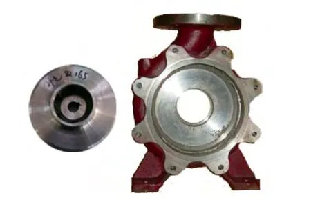
Fig. 1. Impeller and casing of test pump

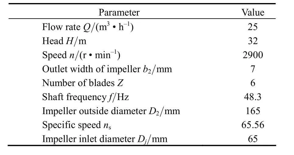
Table 1. Performance and structural parameters of test pump

The noise properties of the centrifugal pump were predicted through a hybrid method using CFD and the Lighthill acoustic analogy theory. In this analogy, the noise sources are divided into three kinds: monopole, dipole, and quadrupole[11]. JIANG, et al[12], indicated that the dipole acoustic source plays a major role in centrifugal pumps with a low specific speed. LANGTHJEM, et al[8–9],assumed that the surface pressure of the impeller is the main noise source in pumps. In accordance with the arguments of these two researchers, the acoustic source in the test pump was simplified to a rotating dipole that is induced by the impeller in this study. The noise at the BPF is the primary component of flow-induced noise in pumps.Thus, the flow-induced noise at the BPF caused by a rotating dipole was calculated to characterize the sound field of flow-induced noise.

Fig. 2 shows the simulation process. During the prediction, the surface pressure pulsations of the blades as provided by ANSYS-CFX are input as a rotating dipole source, and the acoustic field is simulated with the commercial software LMS Virtual Lab Acoustics.

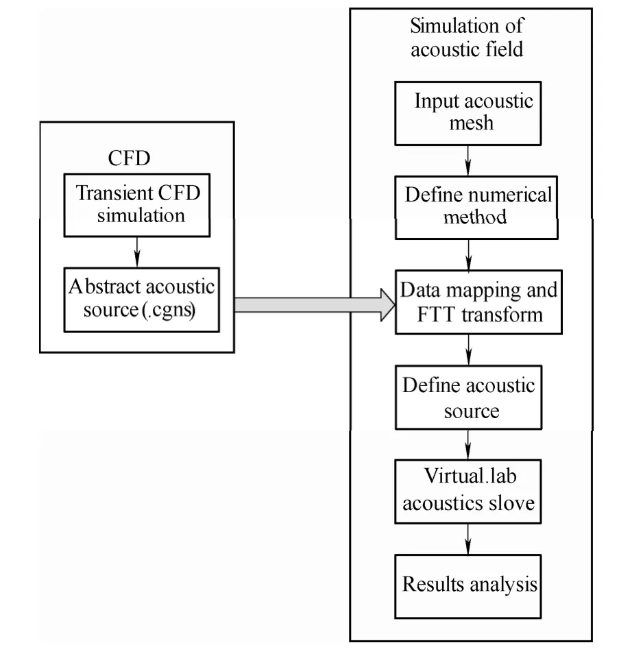
Fig. 2. Process of noise prediction

2.1 CFD model

The acoustic sources were picked from the transient CFD simulation results, so a CFD simulation was done first. In order to calculate the flow field, a 3D map of the test pump was built using Pro/Engineer (Fig. 3). The computational domain of CFD was divided based on the 3D map: a suction duct, extended segment of suction, seal ring, front sidewall gap, impeller, gap between impeller and volute, rear sidewall gap, volute, and outlet duct. In contrast with other numerical models, an extended segment of suction, seal ring, front sidewall gap, and rear sidewall gap were added to account for the effects of the volumetric loss. The grid was generated using ANSYS ICEM CFD Tetra (grid generating software attached to ANSYS). Simulations were performed for five flow rates corresponding to about 60%, 80%, 100%, 120%,and 140% of the design flow rate (Qd). Most of Y plus the value on the blade surface was below 200.

Before the transient simulation, the steady-state calculation was performed first using a frozen-rotor interface between the rotating and stationary zones. A k–ε turbulence model was used. The mass flow rate and static pressure were given as the inlet and outlet boundary conditions at different flow rates. The convergence criteria were set as follows: RMS was chosen as the residual type,and the residual target was 10–4. After the simulation achieved convergence, the steady result was input as an initial condition to start the transient simulations. During the transient solving process, the transient rotor interface was applied instead of the frozen-rotor interface. The unsteady time step was 1.15×10–4s, which was equal to 1/30 of the period for one blade passage when the pump was operating at 2900 r/min. The surface pressure of the blades was output as a CGNS file, which can be input to LMS Virtual Lab as the acoustic source.

Fig. 3. 3D model of test pump

2.2 Model of acoustic prediction

Both the finite element method (FEM) and boundary element method (BEM) were used to simulate low-frequency noise. Of the two, BEM has the advantages of less input data and shorter calculation time. Therefore,BEM was chosen to simulate the rotating dipole sound field made by the impeller in the centrifugal pump.

The direct boundary element method (DBEM) was used to model noise emanating from the impeller source in the pump. During the analysis, the discretization error was often characterized as related to the maximum frequency for which “reasonably accurate” results can be obtained.For boundary elements, this was usually assumed to be the frequency for which there were six elements per wavelength. In other words, the largest element side length in the model was less than or equal to one-sixth of the wavelength. Therefore, the acoustic length of the grid must be valid for the following formula[13]:

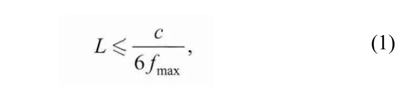
where L represents the side length of element, the maximum frequency fmaxwas 2900 Hz in this case, and the speed of sound in water is c=1483 m/s. Thus, L≤0.085 223 m.The total number of acoustic meshes (Fig. 4) was 11 864,and the length of the largest elements was much less than 0.085 223 m. Therefore, the acoustic mesh was suitable for simulation.

The surface pressure pulsations of the blades were defined as a fan source in the prediction. Each blade was subdivided into a set of sub-segments, and every sub-segment could be replaced by an equivalent source,which was the integration of the pressure pulsations over each surface.

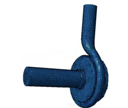
Fig. 4. Acoustic mesh of test pump

3 Experiment Comparison

In order to validate the effectiveness of the simulation, a series of corresponding experiments was conducted. The experimental system comprised a test loop and signal processing system, as shown in Fig. 5. Various operating points were obtained by the test loop. The test signals were received by an NI-PXI-6251 data acquisition card and processed by the relevant module of LABVIEW Express.

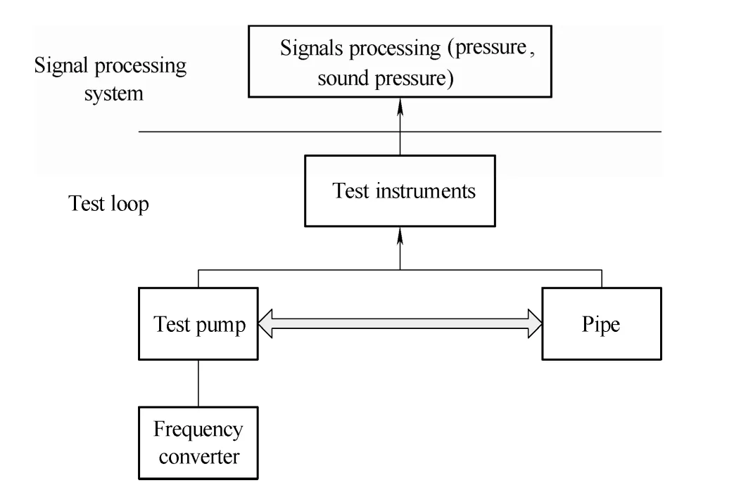
Fig. 5. Composition of experimental system

3.1 Hydrodynamic performance test

The test loop was established as shown in Fig. 6. The medium for this test was clean water at 20 °C. This test loop mainly comprised a motor, test pump, pipe system,flow meter, butterfly valve, hydrophones, and pressure sensors.

For this test, the flow rate Q was measured by the turbine flow meter, which had an accuracy of ±0.3% and standard output signal of 0–5 V. The speed was measured with PROVA RM-1500. The inlet and outlet pressures (psand pd)of the test pump were simultaneously collected by CYG1401 pressure sensors.

These hydraulic parameters were used to plot the performance curve shown in Fig. 7. This figure shows that the best efficient point (BEP) was reached when the flow coefficient KQ=1.9, which is 1.2 times the design flow rate(Qd). The head coefficient KHand flow coefficient KQare formulated as follows:

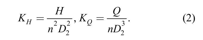
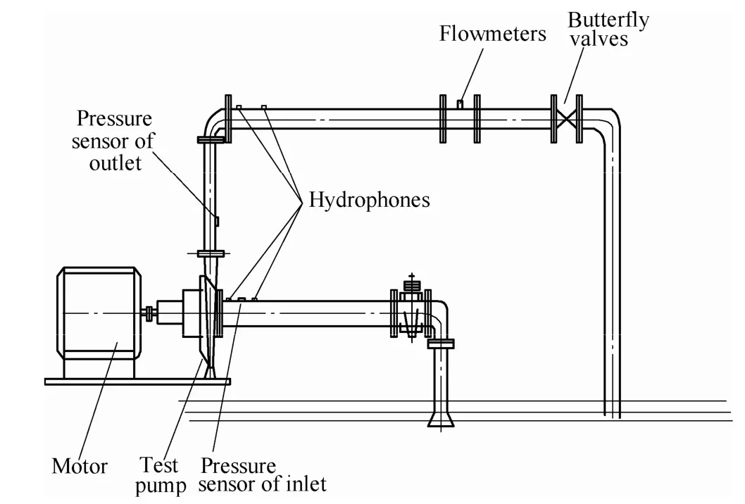
Fig. 6. Diagram of test loop

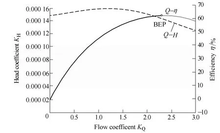
Fig. 7. Performance curve of test pump

3.2 Acoustic test

A four-port model was used to measure the flow-induced noise. Fig. 8 shows a diagram of the four-port model.Coupling between the field variable at the inlet and outlet suctions of the pump was considered for the test model.The test loop was assumed to be one-dimensional, and the sound wave was taken as the superposition of two reverse waves (incident wave p+and reflected wave p–).

The sound pressure in the test was received by B&K8103 hydrophones 1–4 in Fig. 8.and po–represent the incident and reflected waves at the inlet of the test pump and the incident and reflected waves at the outlet,respectively. ps+and ps–were assumed to be the sound of the test pump.

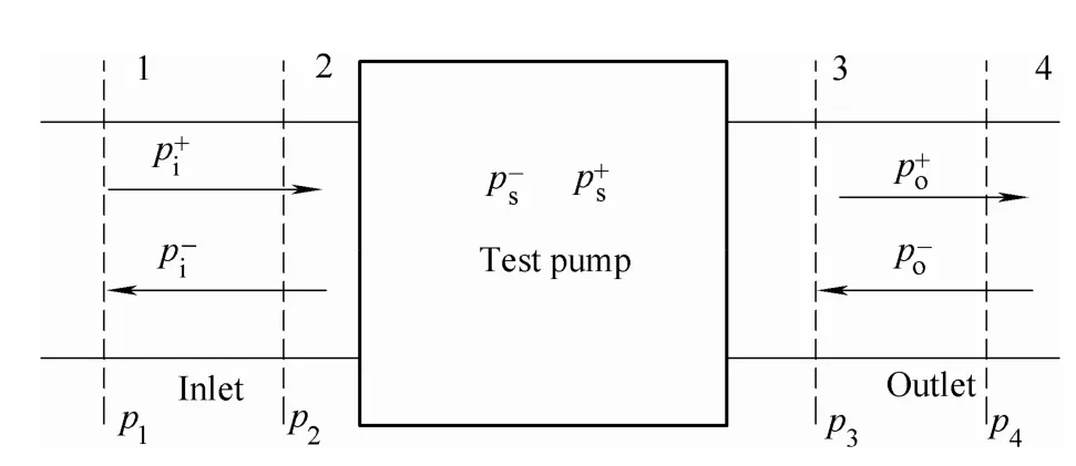
Fig. 8. Diagram of four-port model

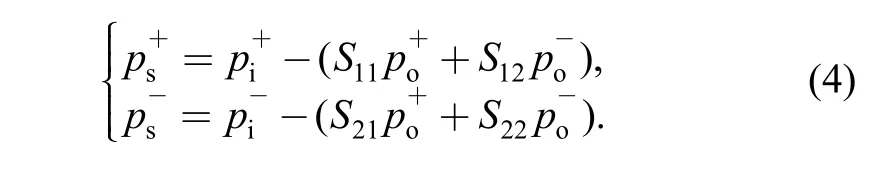
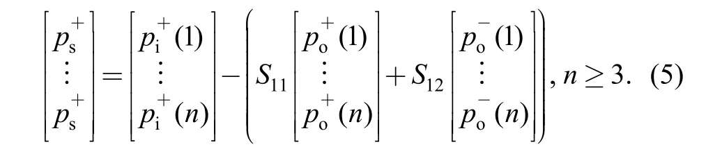
The relationship among them can be expressed as:

where S11, S12, S21, and S22are the transfer matrix elements.Eq. (3) was solved directly and can be rewritten as

The incident and reflected wave components can be experimentally determined from sound pressure measurements at two locations. Therefore,andwere determined from hydrophones 1–4.

Based on the Nyquist sampling theorem and the required test range for flow-induced noise, the sampling interval and sample number were taken as Δt=5×10–5s and N=10 000,respectively.

3.3 Spectrum of pressure and noise in experiment

The pressure and noise signals of the test pump were recorded in the experiment. In this test, the pressure signals at the inlet and outlet of the pump were collected to calculate the performance curves. For the test pump, the pressure pulsations in the pump casing were also examined[15]. The pressure signals were recorded by CYG1145 dynamic pressure transducers on the casing of the test pump. Fig. 9 presents an example of the test pressure amplitude spectra in the pressure experiments. The sound pressure level was calculated by the four-port model presented in section 3.2. The amplitude spectrum of the sound pressure level at Qdis shown in Fig. 10. These two figures show a peak at the shaft frequency that may be closely related with the flow rate, machining precision and quality, dynamic unbalance of impeller, etc. However, the most remarkable spike was at fBPF. In addition, there were some well-defined peaks that corresponded to fBPF, which is mainly induced by the blade-cutoff interaction.

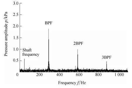
Fig. 9. Pressure amplitude spectra of test pump

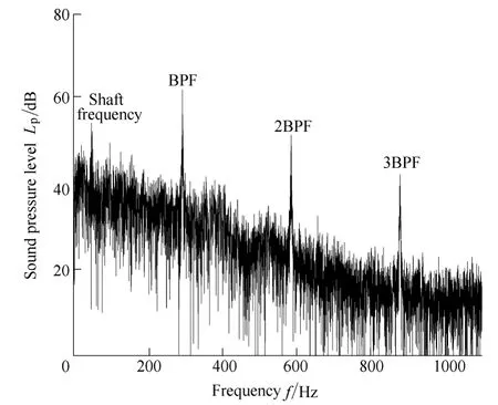
Fig. 10. Sound pressure level amplitude spectra of test pump

4 Results and Discussion

In order to validate the CFD and noise prediction method,the simulation results were compared with the experimental data. Fig. 11 compares the numerical and experimental head–capacity curves and shows the flow rates shifting relative to each other. The CFD results were lower than those of the experimental data. At low and medium flow rates, the difference between the experiment and simulation results was slight. When the flow rate was increased, the gap between these two values increased. However, the relative error was less than 5%. Thus, the numerical results and experimental data showed good agreement with each other.

4.1 Descriptions of pressure pulsations in near-cutoff region

Previous studies analyzed pressure pulsations to research BPF noise[16–18]. In centrifugal pumps, the impeller blade wake flow is a relatively weak primary source, whereas the cutoff in the near field of the impeller acts as a strong secondary source. The acoustic energy radiating from this secondary source depends on the intensity of the velocity and pressure variations it produces. Therefore, the velocity field and pressure pulsations in the near-cutoff region were examined.

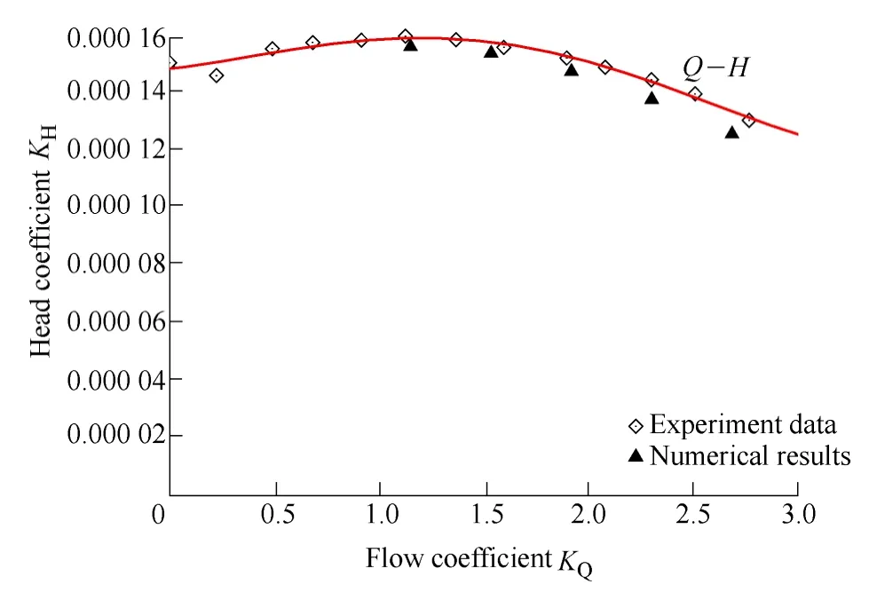
Fig. 11. Comparison of numerical and experimental head–capacity curves

When a couple of impeller blades pass by the tongue, the fluid between them is gradually blocked, which generates serious velocity and pressure pulses. The velocity near the cutoff is complex, and the velocity field of 0.6Qdwas taken as an example. Fig. 12 shows the absolute velocity around the cutoff under this condition. In this region, some of the fluid crossed the cutoff and flowed back to the volute.

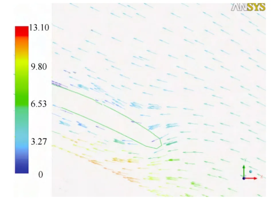
Fig. 12. Velocity field in near-cutoff region under 0.6Qd (m/s)

Fig. 13 includes the pressure contours around cutoff for the other four disparate operating points: 0.8Qd, Qd, 1.2Qd,and 1.4Qd. The pressure field differed at these operating points, but these contours all revealed that the distribution was considerably uneven in the near-cutoff region.

Fig. 13 only shows the pressure distribution in the near-cutoff region in order to highlight the intensity of pressure pulsations.defines the strength of pressure pulsations[19]:

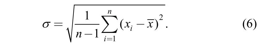
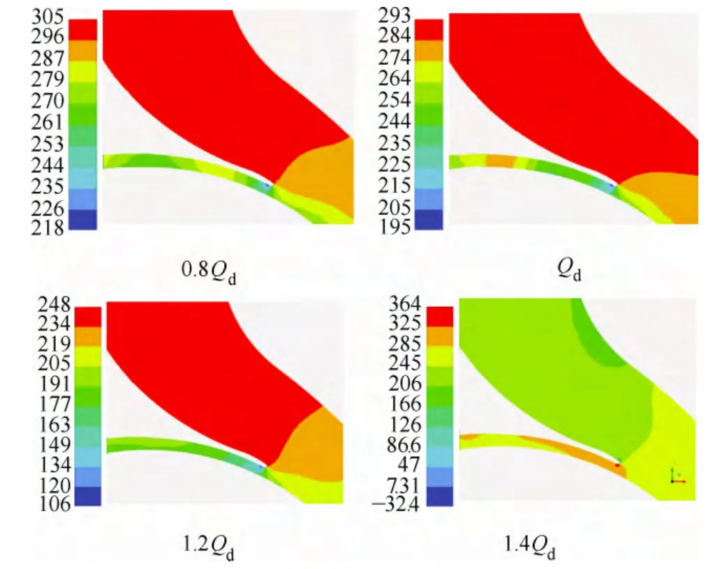
Fig. 13. Pressure field in near-cutoff region at 0.8Qd, Qd, 1.2Qd, and 1.4Qd (kPa)

The sequence of pressure values was xi=(i=1, 2,…, n),andwas the average value of the pressure pulsations.

The observer points in this region were set as shown in Fig. 14. The pressure data of these points were processed using Eq. (6). Fig. 15 shows the bar graph for design point Qd. The graph shows that the strength of the pressure fluctuation was minimum at point g01 near the cutoff. At Qd, the points behind the cutoff had stronger fluctuant strength. This is because, in the near-cutoff region, the flow fluid has strong rotor/stator interactions (RSI) that produce a complex unsteady flow in this region. At medium and low flow rates, this is mainly due to the jet-wake pattern, which is the secondary flow between the pressure and suction sides of the blades. The counter-rotating vortex also has an effect during pump operation at low flow rates[20]. These phenomena result in the maximum pressure taking place near the cutoff; this location differs for different flow rates.

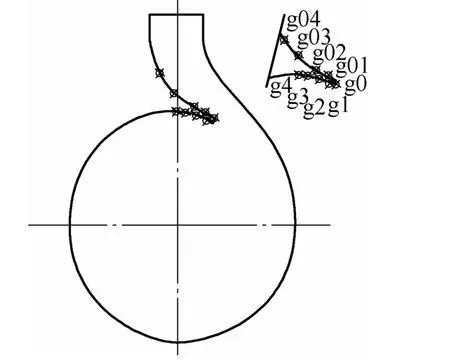
Fig. 14. Pressure observer points of volute in simulation

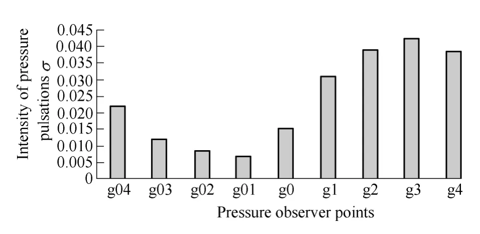
Fig. 15. Bar graph chart of pressure at design point (Qd)

4.2 Calculation results and comparison with experimental data

The features of the inner sound field due to the surface pressure of the impeller were examined at five separate operating points. In order to highlight the differences among these conditions, 15 observer points were set in the simulation, as shown in Fig. 16. Fig. 17 shows the sound pressure distributions of the monitoring points at BPF for these five different operating points, where 0° is the cutoff position. The dipole source characteristics “∞” is obviously in this picture.

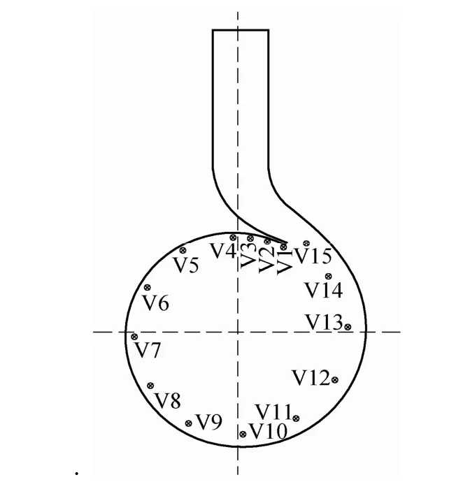
Fig. 16. SPL observer points of pump

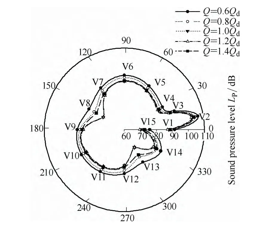
Fig. 17. SPL distributions of observer points

At the same time, there appear other peaks of pressure level due to the interaction with cutoff. However, the peaks of sound pressure level (SPL) were not obtained in V1 where the point was nearest to cutoff while reached nearby V2 and V14. This phenomenon is rather similar to the trend for the pressure strength in the near-cutoff region. This, the flow-induced noise at BPF is directly associated to the intensity of the pressure variations from the second acoustic source.

Fig. 17 shows that the SPL distribution was largest with the low flow rate point (0.6Qd). When the flow was increased to 0.8Qd, the SPL was significantly reduced.Further increasing the flow rate continued to decrease SPL,but the trend became weaker. SPL decreased very slightly between 1.0Qdand 1.2Qd. However, SPL increased significantly when the operation flow was greater than BEP(1.2Qd). Consequently, the simulation results show that the SPL decreased at first but increased with further increases in the flow rate.

These results can be explained through analysis of the internal flow in the pump. At low flow rates, the pump has a turbulent flow field (recirculation, vortex, etc) that causes significant noise. Fig. 18 shows a low pressure distribution near the inlet of the impeller that may be caused by inlet recirculation.

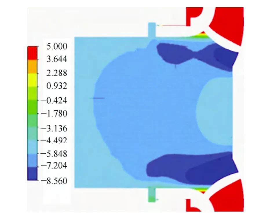
Fig. 18. Pressure distribution (kPa) at inlet of impeller (0.6Qd)

Fig. 19 indicates 2D stream lines along the radial plane of the pump at 0.6Qd, Qd, and 1.2Qd. Fig. 19(a) shows that not only inlet recirculation but also vortexes in the impeller and outlet occurred at 0.6Qd. When the flow rate was increased, the blade flow angle increased and the angle of attack decreased. The trend of stream lines at the radial plane became better at Qd, as shown in Fig. 19(b). There were no vortexes in the impeller, and the vortex was weaker in the outlet. When the flow rate was further increased, the centrifugal pump operated in the high-efficiency zone; the flow field became more stable, as shown in Fig. 19(c), and the vortex in the outlet tended to disappear. Therefore, in the efficient area, the noise decreased slightly with the steady flow field. The noise strength was lowest at 1.2 times the design flow rate.Further increasing the flow rate worsened the flow field,and cavitation became serious, so more noise was caused than at 1.2Qd.

The predicted acoustic results were verified using the experimental results. The specific process for the experimental data is presented below. The measured sound pressure level was Lpand is calculated as follows[21]:

where p represents the measured sound pressure. prefis the reference sound pressure and was 2×10–5Pa.

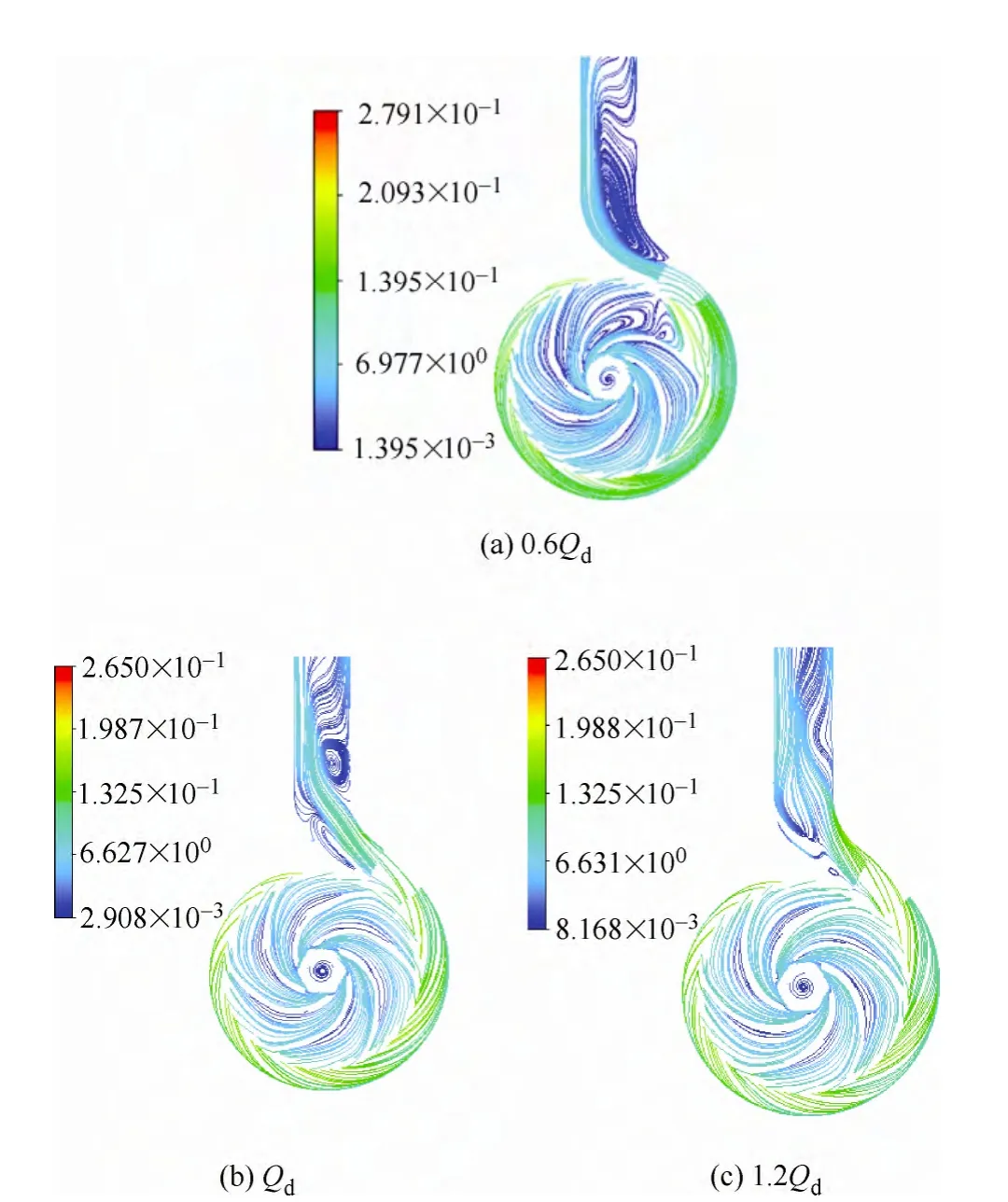
Fig. 19. Stream lines at radial plane of test pump (m/s)

The incident and reflected waves in the test pump were calculated with the four-port model; the details on the calculation are given in section 3.2. The sound pressure at each operating point is expressed by the following formula:

Fig. 20 shows the test SPL corresponding to different operating points. When compared with Fig. 17, the flow rates that correspond to the maximum and minimum SPL of the numerical and experiment data were consistent with each other. However, from 0.8Qdto the design condition(Qd), the reduction of SPL was not clear in the experiment compared with the marked drop in the simulation. Possible reasons for the difference are listed as follows. First, there is a certain error in the experimental results. Every step of the experiment may have an error, including errors with the method, device, and data processing. Second, the acoustic source was simplified for noise prediction. The effects of monopole and quadrupole noise sources on the acoustic field would be stronger when the pump operating drifts off the BEP, which would decrease the accuracy of the simulated noise.

Although there were some differences between the results from the experiment and numerical simulation, the trends were consistent. Thus, the simulation can be used to optimize the design of low-noise centrifugal pumps.

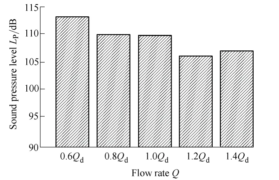
Fig. 20. Test SPL under different flow rate conditions

5 Conclusions

A numerical scheme was designed to quickly optimize low-noise centrifugal pumps in actual projects and used to simulate the acoustic trend of flow-induced noise in a pump with flow migration. In this numerical simulation, the flow-induced noise at BPF made by a rotating dipole is used to characterize the flow-induced acoustic field. It was combined with LMS Virtual Lab Acoustic and CFX. Only the acoustic field at BPF is calculated, which reduces the computation cost and shortens the calculation time. Five different operating points were simulated, and the simulation results for the flow and acoustic field were analyzed. Comparison with the experimental results showed the following:

(1) Analysis of pressure pulsations and the SPL distribution at BPF in the near-cutoff region showed that the hybrid method of CFD coupled with computational acoustic can predict the flow-induced noise at BPF that is induced by rotor-stator interaction.

(2) The noise prediction indicated that the SPL decreased with increasing flow mass when the pump operated at low and medium flow rates and reached its lowest value near BEP (1.2Qd). The SPL then increased with further increasing of flow rate. This trend compared well with the trend obtained by the experiment.

Thus, the flow-induced acoustic features in the model pump are roughly reflected by the flow-induced noise at the BPF, which is generated by the blade-rotating dipole.However, the deviation increases as the operating condition becomes further away from the rated condition. When the operating condition is sufficiently far from the rated condition, the influence of other unsteady flow phenomena(rotating stall, cavitation, reverse flow, etc) becomes too strong to ignore. As a result, the numerical scheme method is not suitable in that situation. Thus, the next step of this research will involve considering the influence of other unsteady flow phenomena to broaden the applicability of this numerical scheme.

[1] BERND D, FRANK-HENDRIK W. Noise sources in centrifugal pumps[C]//Conference on Applied and Theoretical Mechanics,Venice, Italy, 2006: 203–207.

[2] JEON W. A numerical study on the effects of design parameters on the performance and noise of a centrifugal fans[J]. Journal of Sound and Vibration, 2003, 265(1): 221–230.

[3] SEUNGYUB L, SEUNG H, CHELUNG C. Prediction and reduction of internal blade-passing frequency noise of the centrifugal fan in a refrigerator[J]. International Journal of Refrigeration, 2010, 33(6): 1129–1141.

[4] CHOI J S, MCLAUGHLIN D K, THOMPSON D E. Experiments on the unsteady flow field and noise generation in a centrifugal pump impeller[J]. Journal of Sound and Vibration, 2003, 263(3):493–514.

[5] LI You, OUYANG Hua, TIAN Jie, et al. Experimental and numerical studies on the discrete noise about the cross-flow fan with block-shifted impellers[J]. Applied Acoustic, 2010, 71(12):1142–1155.

[6] JONG-SOO C, DENNIS K, MCLAUGHLIN D E. Experiments on the unsteady flow field and noise generation in a centrifugal pump impellers[J]. Journal of Sound and Vibration, 2003, 263(3):493–514.

[7] WILLIAM Layton, ANTONIN Novotny. ON Lighthill’s acoustic analogy for low Mach number flows[J]. Advances in Mathematical Fluid Mechanics, 2010: 247–279.

[8] LANGTHJEM M A, OLHOFF N. A numerical study of flow-induced noise in a two-dimensional centrifugal pump-PartⅠ:hydrodynamics[J]. Journal of Fluids and Structur., 2004, 19(3):349–368.

[9] LANGTHJEM M A, OLHOFF N. A numerical study of flow-induced noise in a two-dimensional centrifugal pump part ii.hydroacoustics[J]. Journal of Fluids and Structures, 2004, 19(3):369–386.

[10] SERGEY T. Development and experimental validation of 3D acoustic-vortex numerical procedure for centrifugal pump noise prediction[C/CD]//Proceedings of the ASME 2009 Fluids Engineering Division Summer Meeting, 2009, Colorado, USA,FEDSM2009-78400.

[11] LIGHTHILL M J. On sound generated aerodynamically. I. General theory[C]//Proceeding of the Royal Society of London, SERIES A.Mathematical and Physical Science, 1952, 211 (1107): 564–587.

[12] JIANG Y Y, YOSHIMURA S, IMAI R. Quantitative evaluation of flow-induced structural vibration and noise in turbomachinery by full-scale weakly coupled simulation[J]. Journal of Fluids and Structures, 2007, 23(4): 531–544.

[13] LI Zenggang, ZHAN Fuliang. LMS virtual lab acoustic the advanced applications of acoustic simulation[M]. Beijing: National Defence Industry Press, 2010. (in Chinese)

[14] FENG Tao. The measurement study of the flow-induced noise in centrifugal pumps[D]. Beijing: Institute of Acoustics, China Academy of Sciences, 2003. (in Chinese)

[15] ZHU Lei. Study on rotor-stator interaction of a centrifugal pump based on LES and experiments of the pressure fluctuation[D].Zhenjiang: Jiangsu University, 2011. (in Chinese)

[16] TALHA A, BARRAND J P, CAIGNERT G. Pressure fluctuations on the impeller blades of a centrifugal turbomachine: a comparative analysis between air and water tests[J]. Int. J. Acoust. Vib., 2002,7(1): 45–51.

[17] JORGE P, JAVIER P, RAÚL B, et al. A simple acoustic model to characterize the internal low frequency sound field in centrifugal pumps[J]. Applied Acoustic, 2011, 72(1): 59–64.

[18] RZENTKOWSKI G. Generation and control of pressure pulsation emitted from centrifugal pump[C]//ASME PVP Conference,Montreal, Canada; 1996, 328: 439–454.

[19] SONG Zhenghua, ZHOU Jiren, TANG Fangping. Acquisition and analysis of signals in tubular pump pressure pulsation test[J].Journal of Yangzhou University (Natural Science Edition), 2009,12(2): 53–57. (in Chinese)

[20] RAÚL B, JORGE P, EDUARDO BLANCO. Numerical analysis of the unsteady flow in the near-tongue region in a volute-type centrifugal pump for different operation points[J]. Computers &Fluid, 2010, 39(5): 859–870.

[21] DU Gonghuan, ZHU Zheming, GONG Xiufeng. The basis of acoustics[M]. Nanjing: Nanjing University Press, 2001. (in Chinese)