一类概括化位置不变重尾指数估计

刘维奇，张丹青

（1.山西大学 数学科学学院，山西 太原 030006；2.山西大学 管理与决策研究所，山西 太原 030006）

0 引言

假设X1，…，Xn是一列独立同分布的随机变量序列，具有共同的分布函数F，设X1，n≤…≤Xn，n为其递增的次序统计量。若F∈D（Gr），则存在常数列an＞0，bn∈R，对任意的x∈R，当n趋于无穷时，有P，其中

由于对极端事件的关注，重尾现象出现在越来越多的领域，如，金融学，保险业，计算机科学，水文学以及气象学等，为了了解尾部的全部信息，故对重尾指数γ的估计也就成了重中之重。事实上，学者们对重尾指数γ的估计也进行了广泛的研究，如要求γ＞0的Hill估计［1］，Hill估计具有强相合性和渐近正态性［2］。根据Hill估计，Dekkers等［3］提出了适用于γ∈R的矩估计，并在（1）式二阶正则条件下证明其渐近性质

此时，γ＞0，ρ＜0，A（t）∈RVρ.又如Pickands提出的 Pickands估计［4］，Davison［5］的极大似然估计，Csorgo等［6］的核估计，Fraga Alves等［7］提出的 MM 混合矩估计，Kratz和 Resnick［8］提出的qq－plot估计，Gomes和Martins［9］提出的 GJ估计，Beirlant等［10］提出的广义 Hill估计，Gomes等［11－12］提出的修正 CM 估计，Davydov等［13］提出的DPR样本分块估计等等，刘维奇，邢红卫在此基础上进一步阐明了重尾指数估计的研究进展［14］，位置不变和降偏差成为尾指数近年来研究的热点，如Brahim等［15］的降偏差估计，本文提出的估计量是基于Gomes和 Martins［16］提出的概括化估计量：

在上述经典估计中，位置不变的估计量很少，大部分估计均是非位置不变的，即对样本进行位置变换后不满足位置不变性，而在实际问题中，我们往往需要对样本进行位置变换。因此，位置不变的重尾估计也就成为重尾研究的热点之一。如Frage Alves［17］提出的位置不变的Hill估计，

Ling等［18－19］提出的位置不变矩估计：

其中，

收敛于Γ（α＋1）γα，而k0和k是整数序列，也就是说，

类似的还有Li等［20－21］提出的一类位置不变的Hill型估计。除以上方法外，还有学者用X＊i＝Xi－X［np］＋1，n，（0≤p＜1，1≤i≤n）来代替原始样本Xi，如 Araujo Santos等［22］提出的几类位置不变重尾估计，称为PORT（Peaks Over Random Threshold）方法，及Gomes等［11－12］提出的估计，Fraga和 Gomes等［7］提出的位置不变混合矩估计，此外还有Falk［23］提出的NH估计，Peng和Nadarajah［24］提出的 Weiss类Pickands估计等，而Ling等［25］则巧妙地结合了两种位置不变估计，本文利用统计量M（α）n（k0，k）和Gomes，Martin［16］中的估计提出一类新的概括化位置不变的重尾指数估计

1 主要结果

其中，RVβ表示在无穷远处极值指数β的一类正则变化函数。为了方便理论计算的证明，做如下记号：

为了研究估计量的渐近性质，我们还需如下二阶条件：假设存在函数a（t）＞0，可测函数＝0，有［26］，

表1 α＝α0γ ＝ α0∶b－γα ＝0Table 1 α＝α0（γ）＝｛α0∶b（－γ，α）＝0｝

2 模拟研究

图1表示估计量无偏时，即b（－γ，α）＝0，知α0（γ）是γ的减函数，并在表1中列举了几种特殊的γ值和其对应的α0（γ）值以便后面更进一步的研究。

Fig.1 （1＋γ）1－α0＋γ（α0－2）＝1图1 （1＋γ）1－α0＋γ（α0－2）＝1

接下来，选择Burr（1，－1）模型，当b（－γ，α）＝0时，由表1得出α0（1）＝2.7，选取样本量为2 500，α的值为1，2，2.7，4，分别比较画出（k0，k）（k0，k），（k0，k），和（k0，k）的路径图，由图2可以看出α0（1）＝2.7蓝色的线有最小的偏差，效果最好，与γ的真值最接近。

Fig.2 Sample paths of（k0，k）（k0，k）（k0，k），and（k0，k）for Burr（1，－1）model with sample size n＝2 500图2 Burr模型下，样本2 500时（k0，k），＾（k0，k）（k0，k）（k0，k）的样本路径图

由定理1.2我们得到γnk0k的渐近偏差与渐近方差：

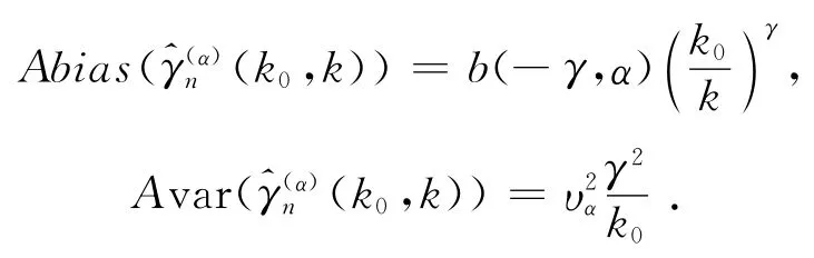
图3中，上图可以看出，对于每一个固定的α，随着γ的增大，b（－γ，α）越来越小；同样，由下图可以看出，对于每一个固定的γ，随着α的增大，b（－γ，α）先减小再增大。

Fig.3 b（－γ，α）as a function ofγ（up）andα（down）图3 b（－γ，α）分别于γ（上）和α（下）的函数图像

Fig.4 Image of Squared Bias b2（－1，α）（left）and Variance（right）of（k0，k）图4 （k 0，k）偏差平方b2（－1，α）（左）和方差（右）的图像

图5为Frechet，Burr和Pareto三种分布模型下）（虚线）的路径图。取5 000个随机数，令，由于k≤16时，k＜k0，而k0是从k中选取的，故k＞k0，所以我们不考虑图中前一小部分的异常值，从k≥17来看（k0，k）的稳健性相当好，几乎接近于真值。

图6同样表示在Frechet（2）模型下，将1 500个样本复制500次，分别模拟出新估计量（k0，k）与传统经典位置不变估计量（k0，k）和（k0，k）的均值和均方误差，新估计量的模拟结果最好，类似的研究如图7和图8。

Fig.5 Sample paths of（k0，k）（solid line）and（dotted line）for Frechet（left），Burr（middle）and Pareto（right）withα＝2.7图5 α＝2.7时，三种分布Frechet（左），Burr（中）和 Pareto（右）下＾（k0，k）（实线）和（k）（虚线）的样本路径图

表2 Frechet（2）模型下（k0，k）的MSETable 2 MSE of（k 0，k）for Frechet（2）model

表2 Frechet（2）模型下（k0，k）的MSETable 2 MSE of（k 0，k）for Frechet（2）model

2.4 100 0.142 8 0.112 38 0.119 11 0.129 39 0.144 14 0.n α＝1 α＝1.3 α＝1.4 α＝1.5 α＝1.8 α＝2 α＝146 41 0.167 13 200 0.071 733 0.061 121 0.058 653 0.074 096 0.088 059 0.095 715 0.121 85 300 0.051 492 0.046 104 0.043 908 0.054 046 0.067 707 0.075 477 0.100 46 400 0.044 2 0.040 185 0.034 834 0.046 941 0.057 409 0.063 704 0.088 653 500 0.045 064 0.034 365 0.029 281 0.041 439 0.049 067 0.055 774 0.078 601 600 0.040 129 0.031 033 0.027 877 0.038 802 0.043 867 0.050 554 0.071 08 700 0.038 835 0.031 532 0.026 943 0.036 013 0.040 067 0.046 865 0.065 743 800 0.038 282 0.032 458 0.025 244 0.034 047 0.03 6 072 0.041 814 0.056 687 1 000 0.035 589 0.032 888 0.025 34 0.031 617 0.03 7 681 0.043 816 0.060 054 900 0.037 977 0.033 308 0.025 184 0.032 705 0.03 4 421 0.040 11 0.052 109

Fig.6 Mean value and MSE of（k0，k），（k 0，k）and（k 0，k）for Frechet（2）model with sample size n＝1 500 and 500 replications图6 Frechet（2）模型下，样本量n＝2 500时（k0，k），（k 0，k）（k0，k）的均值和均方误差

表3 Burr 1－1模型下k 0 k 的MSETable 3 MSE of（k0，k）for Burr（1，－1）model

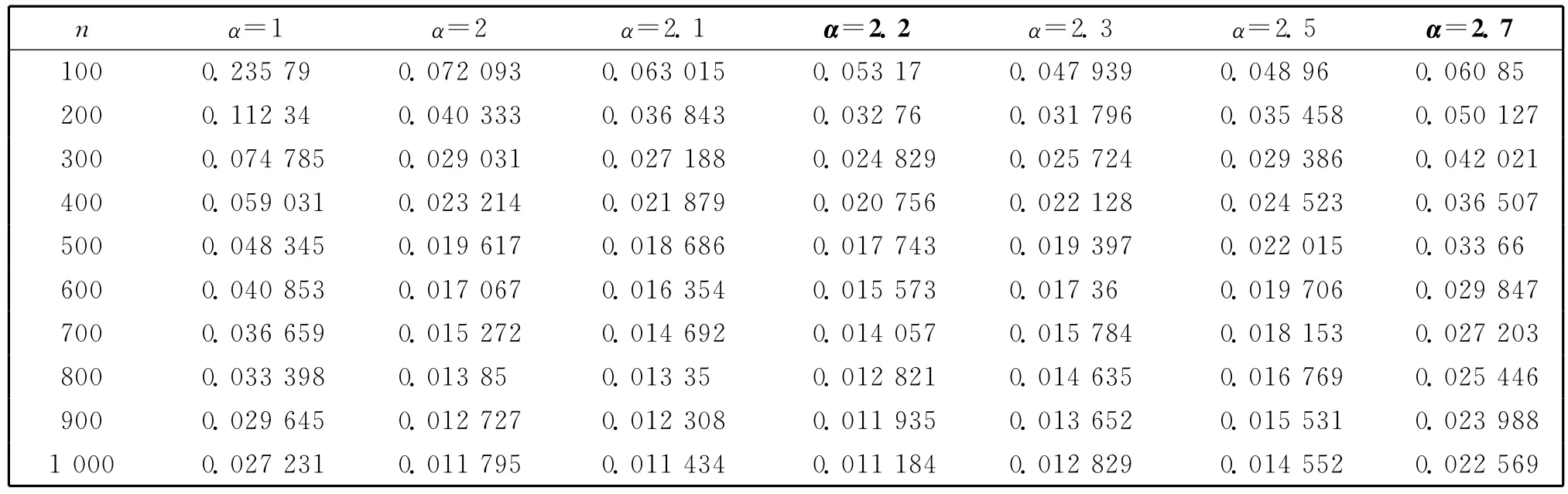
表3 Burr 1－1模型下k 0 k 的MSETable 3 MSE of（k0，k）for Burr（1，－1）model

2.7 100 0.235 79 0.072 093 0.063 015 0.053 17 0.047 9 n α＝1 α＝2 α＝2.1 α＝2.2 α＝2.3 α＝2.5 α＝39 0.048 96 0.060 85 200 0.112 34 0.040 333 0.036 843 0.032 76 0.031 796 0.035 458 0.050 127 300 0.074 785 0.029 031 0.027 188 0.024 829 0.025 724 0.029 386 0.042 021 400 0.059 031 0.023 214 0.021 879 0.020 756 0.022 128 0.024 523 0.036 507 500 0.048 345 0.019 617 0.018 686 0.017 743 0.019 397 0.022 015 0.033 66 600 0.040 853 0.017 067 0.016 354 0.015 573 0.017 36 0.019 706 0.029 847 700 0.036 659 0.015 272 0.014 692 0.014 057 0.015 784 0.018 153 0.027 203 800 0.033 398 0.013 85 0.013 35 0.012 821 0.014 6 3 652 0.015 531 0.023 988 1 000 0.027 231 0.011 795 0.011 434 0.011 184 0.0 35 0.016 769 0.025 446 900 0.029 645 0.012 727 0.012 308 0.011 935 0.01 12 829 0.014 552 0.022 569

Fig.7 Mean value and MSE of（k0，k）（k0，k）and（k0，k）for Burr（1，－1）model with sample size n＝1 500 and 500 replications图7 Burr（1，－1）模型下，样本量n＝2 500时（k0，k）（k 0，k）（k0，k）的均值和均方误差

表4 Pareto（0.5）模型下（k 0，k）的MSETable 4 MSE of（k0，k）for Pareto（0.5）model

表4 Pareto（0.5）模型下（k 0，k）的MSETable 4 MSE of（k0，k）for Pareto（0.5）model

3.2 100 0.399 84 0.138 2 0.049 927 0.022 689 0.010 80 n α＝1 α＝2 α＝2.5 α＝2.9 α＝3 α＝3.1 α＝2 0.014 763 0.016 534 200 0.216 04 0.083 452 0.032 163 0.016 932 0.006 8153 0.0103 49 0.015 522 300 0.169 04 0.065 0.026 146 0.014 385 0.005 8638 0.009 631 0.013 017 400 0.143 1 0.054 25 0.022 544 0.013 092 0.005 338 0.009 040 0.012 165 500 0.127 55 0.047 639 0.020 37 0.011 213 0.004 863 8 0.008 607 0.010 213 600 0.109 87 0.043 025 0.018 99 0.010 397 0.004 465 9 0.007 458 0.010 314 700 0.098 987 0.039 601 0.017 506 0.009 724 4 0.004 163 3 0.006 921 0.009 581 800 0.089 145 0.036 55 0.016 586 0.009 175 6 0.00 03 838 6 0.006 545 0.008 251 1 000 0.077 517 0.032 3 0.014 664 0.007 939 7 0.00 3 949 7 0.006 540 0.008 279 900 0.082 474 0.034 461 0.015 429 0.008 559 2 0.0 3 622 4 0.006 390 0.007 840

3 证明

为证明主要结果，我们需要如下结论。

Fig.8 Mean value and MSE of（k0，k）（k0，k）and（k0，k）for Pareto（0.5）model with sample size n＝1 500 and 500 replications图8 Pareto（0.5）模型下，样本量n＝2 500时（k 0，k）（k0，k），（k 0，k）的均值和均方误差

［1］ Hill B.A Simple General Approach to Inference About the Tail of a Distribution［J］.Annals of Statistics，1975，3：1163-1174.

2 de Haan.Extreme Value Statistics C Galambos J Lechner J Simiu E.eds.Extreme Value Theory and Applications Kluwer Academic Publications，Dordrecht，1994：93-122.

［3］ Dekkers A，Einmahl J，de Haan L.A Moment Estimator for the Index of an Extreme-value Distribution［J］.Annals of Statistics，1989，17：1833-1855.

［4］ Pickands J.Statisticla Inference Using Extreme Order Statistic［J］.Annals of Statistics，1975，3：119-131.

［5］ Davison A C.Modelling Excesses Over High Thresholds［C］／／Tiago de Oliveira J.（Ed），Statistical Extremes and Application.Reidel，Dordrecht，1984：461-482.

［6］ Csorgo S，Deheuvels P，Mason D.Kernel Estimates of the Tail Index of a Distribution［J］.Annals of Statistics，1985，13（3）：1050-1077.

［7］ Fraga Alves M I，Gomes M I，de Haan L，et al.Mixed Moment Estimator and Location Invariant Alternatives［J］.Extremes，2009，12：149-185.

［8］ Kratz M，Resnick S.The qq-estimator and Heavy Tails［J］.Stochastic Models，1996，12（4）：699-724.

［9］ Gomes M I，Martins M J.“Asymptotically Unbiased”Estimators of the Tail Index Based on External Estimation of the Second Order Parameter［J］.Extremes，2002，5（1）：5-31.

［10］ Beirlant J，Dierckx G，Guillou A.Estimation of the Extreme Value Index and Generalized Quantile Plots［J］.Bernoulli，2005，11（6）：949-970.

［11］ Gomes M I，Fraga Alves M I，Araújo Santos P.PORT Hill and Moment Estimators for Heavy-tailed Models［J］.Communications in Statistics Simulationand Computation，2008a，37：31-53.

［12］ Gomes M I，Fraga Alves M I，Araújo Santos P.PORT Hill and Moment Estimators for Heavy-tailed Models［J］.Communications in Statistics Simulation and Computation，2008b，37：1281-1306.

［13］ Davydov Y，Paulauskas V，Rackauskas A.More on P-stable Convex Sets in Banach Spaces［J］.Journal of Theoretical Probability，2003，13：39-64.

［14］ 刘维奇，邢红卫.重尾分布尾指数估计研究进展［J］.山西大学学报：自然科学版，2012，5：163-173.

［15］ Brahim B，Djamel M，Abdelhakim N，et al.A Bias-reduced Estimator for the Mean of a Heavy-tailed Distribution with an Infinite Second Moment［J］.Journal of Statistical Planning and Inference，2013，143（6）：1064-1081.

［16］ Gomes M I，Martins M J.Generalizations of the Hill Estimator-asymptotic Versus Finite Sample Behaviour［J］.Statistics Plan Inference，2001，93（1-2）：161-180.

［17］ Fraga Alves M I.A Location Invariant Hill-type Estimator［J］.Extremes，2001，4（3）：199-217.

［18］ Ling C，Peng Z，Nadarajah S.A Location Invariant Moment-type EstimatorⅠ［J］.Theory of Probability and Mathematical Statistics，2007，76：23-31.

［19］ Ling C，Peng Z，Nadarajah S.A Location Invariant Moment-type EstimatorⅡ［J］.Theory of Probability and Mathematical Statistics，2007，77：177-189.

［20］ Li J，Peng Z，Nadarajah S.A Class of Unbiased Location Invariant Hill-type Estimators for Heavy Tailed Distributions［J］.Electronic Journal of Statistics，2008：829-847.

［21］ Li J，Peng Z，Nadarajah S.Asymptotic Normality of Location Invariant Heavy Tail Index Estimators［J］.Extremes，2010，13：269-290.

［22］ Araújo Santos P，Fraga Alves M I，Gomes M I.Peaks Over Random Threshold Methodology for Tail Index and Quantile Estimation［J］.Revstat 4，2006：227-247.

［23］ Falk M.Some Best Parameter Estimates for Distributions with Finite Endpoint［J］.Statistics，1995，27：115-125.

［24］ Peng Z，Nadarajah S.The Pickands’Estimator of the Negative Extreme Value Index［J］.Acta Scientiarum Naturalium Universitatis Pekinensis，2001，37：12-19.

［25］ Ling C，Peng Z，Nadarajah S.Location Invariant Weiss-Hill Estimator［J］.Extremes，2012，15：197-230.

［26］ de Haan，Stadtmüller.Generalized Regular Variation of Second Order［J］.Australian Mathematical Society，1996，61：381-395.

［27］ Peng L.Asymptotically Unbiased Estimators for the Extreme-value Index［J］.Statistics and Probability Letters，1998，38（2）：107-115.