
QUANTILE ESTIMATION WITH AUXILIARY INFORMATION UNDER POSITIVELY ASSOCIATED SAMPLES∗
2016-09-26 03:45YinghuaLI李英华YongsongQIN秦永松QingzhuLEI雷庆祝LifengLI李丽凤
关键词:英华
Yinghua LI(李英华) Yongsong QIN(秦永松)Qingzhu LEI(雷庆祝)Lifeng LI(李丽凤)
Department of Mathematics,Guangxi Normal University,Guilin 541004,China
E-mail∶54503514@qq.com;ysqin@gxnu.edu.cn;qzlei@gxnu.edu.cn;1057171318@qq.com
QUANTILE ESTIMATION WITH AUXILIARY INFORMATION UNDER POSITIVELY ASSOCIATED SAMPLES∗
Yinghua LI(李英华) Yongsong QIN(秦永松)†Qingzhu LEI(雷庆祝)Lifeng LI(李丽凤)
Department of Mathematics,Guangxi Normal University,Guilin 541004,China
E-mail∶54503514@qq.com;ysqin@gxnu.edu.cn;qzlei@gxnu.edu.cn;1057171318@qq.com
The empirical likelihood is used to propose a new class of quantile estimators in the presence of some auxiliary information under positively associated samples.It is shown that the proposed quantile estimators are asymptotically normally distributed with smaller asymptotic variances than those of the usual quantile estimators.
Quantile;positively associated sample;empirical likelihood
2010 MR Subject Classification62G05;62E20
1 Introduction
The empirical likelihood(EL)method as a nonparametric technique for constructing confidence regions in the nonparametric setting was introduced by Owen[1,2].The EL method was used in statistical inferences for quantiles in various contexts such as in the context of independent sample by Chen and Hall[3]and in the case of survey sampling by Chen and Wu[4].The blockwise EL method was first proposed by Kitamura[5]to construct confidence intervals for parameters with mixing samples.A striking feature of the EL is its ability to use auxiliary information.Zhang[6]applied the EL technique to propose a new class of M-functional estimators as well as quantile estimators in the presence of some auxiliary information under independent samples.Chen and Qin[7]shown that the EL method can be naturally applied to make more accurate statistical inference in finite population estimation problems by employing auxiliary information efficiently.Under negatively associated(NA)samples,Qin and Lei[8]obtained the asymptotical distribution of the smooth kernel estimator of a quantile in the presence of some auxiliary information in conjunction with the EL method.
Negative association of random variables occurs in a number of important cases,but it has not been as popular as positive association[9].On the other hand,it is much more difficult technologically to deal with positively associated(PA)samples than NA samples becanse thereexist nice moment inequalities for sums of NA sequences and there are no nice moment inequalities for sums of PA sequences.Thus,it is interesting to work on the quantile estimation with auxiliary information under PA samples.
It is worth mentioning the definition of PA random variables and their applications here. Random variables{ξi,1≤i≤n}are said to be PA,or just associated,if for any real-valued coordinatewise nondecreasing functions f1and g1,

whenever this covariance exists.An infinite family of random variables is associated if every finite subfamily is associated.The concept of PA random variables was introduced by Esary et al[10],which attracts more and more attention because of its wide applications in multivariate statistical analysis and reliability theory;see,for example,Birkel[11-13],Esary et al[10],Bagai and Prakasa Rao[14]
In this article,we apply the EL technique to propose a new class of quantile estimators in the presence of some auxiliary information under PA samples.It is shown that the proposed quantile estimators are asymptotically normally distributed with smaller asymptotic variances than those of the usual quantile estimators.
The rest of this article is organized as follows.The main results of this article are presented in Section 2.Simulations to examine the performance of the proposed quantile estimators are presented in Section 3.Some lemmas to prove the main results are given in Section 4.The proof of the main results is presented in Section 5.
2 Main Results
Throughout this article,we assume that X1,X2,···,Xnis a sequence of PA random variables,and F be the distribution function of their common population X.We also assume that some auxiliary information about the distribution function F is available in the sense that there exist r(r≥1)known functions g1(x),g2(x),···,gr(x)such that

where g(x)=(g1(x),g2(x),···,gr(x))τis an r-dimensional vector.Using the auxiliary information(2.1),we will propose a new class of quantile estimators.
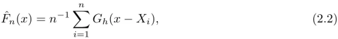
Without the auxiliary information(2.1),the smooth estimator of F is defined as
i=1
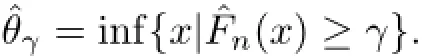
hnAccordingly,the smooth kernel estimator of θγ=:F−1(γ)=inf{x|F(x)≥γ}(0<γ<1)is defined by
Under some dependent samples including PA and NA samples,Cai and Roussas[15]studied the asymptotic normality ofˆθγ.
We will use the auxiliary information(2.1)to obtain a new estimator of θγby the blockwise EL method as follows.Let p=p(n)and q=q(n)be positive integers satisfying p+q≤n,and
k=[n/(p+q)],where[t]denotes the integral part of t.Put

where rm=(m−1)(p+q)+1,lm=(m−1)(p+q)+p+1,m=1,···,k.Define the following blockwise EL function

with λ∈Rrbeing determined by

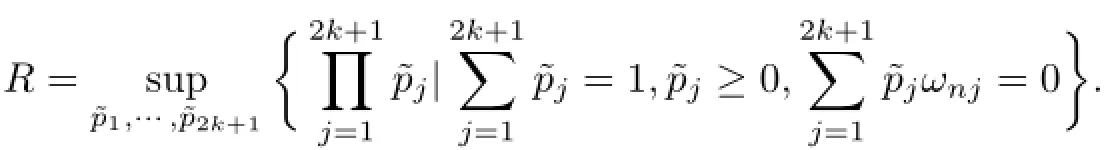
Thus,under auxiliary information(2.1),a new estimator of F(x)at a given x∈R is

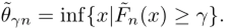
and the new smooth kernel estimator of θγis defined by where with rm=(m−1)(p+q)+1,lm=(m−1)(p+q)+p+1,m=1,···,k.

Assumptions
(A1)(i)The X1,X2,···,Xnform a stationary sequence of real-valued r.v.s.with distribution function F,bounded probability density function f,and f(θγ)>0.
(ii)The Xi's are PA with EX21<∞.
(iv)The derivative f′(x)exists and is bounded in a neighborhood of θγ.
(v)For all x∈R and each j≥2,Fj|1(y|x)is continuous in a neighborhood of θγ,where Fj|1(y|x)is the conditional distribution function of Xjgiven X1.
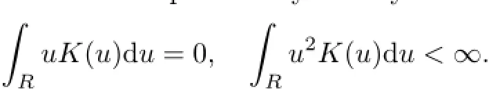
(A2)The function K is a bounded probability density function and satisfies
(A3)The sequence of bandwidths{h=hn,n≥1}satisfies 0<h→0,nh→∞,nh4→0.
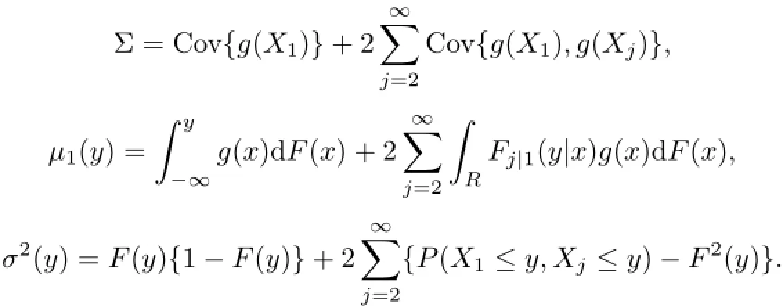
(A4)gj(x),1≤j≤r,have bounded derivatives on R.There is a constant δ>0 such that(X)<∞,Eg(X)=0,E[‖g(X)‖6+2δ]<∞,and Σ>0,where Vgj(x)is the total variation function of gj(x),1≤j≤r,and

(A5)Let p,q,k,and u(n)be as described above,which satisfy
(i)q→∞and q/p→0.
(ii)p2(3+δ)/(2+δ)/n→0.
We now state the main results of this article.
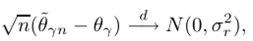
Theorem 2.1Suppose that conditions(A1)to(A5)are satisfied.Then,as n→∞,where with


Remark 2.2From Cai and Roussas[15],√n(ˆθγ−θγ)d−→N(0,σ2(θγ)/f2(θγ)),which implies that the asymptotic variance of˜θγnis less than or equal to that ofˆθγ.
Remark 2.3The choice of the bandwidth is an important issue.There is no satisfactory approach available now.Further study in choosing the bandwidth is surely needed in the case of dependent samples.
3 Simulation Results
We conducted a small simulation to study the finite sample performance of the proposed estimators of quantiles.In the simulation,is an i.i.d.sequence with˜X1~N(0,1).Note that{Xi,1≤i≤n}is an PA sequence[9]. Suppose that we know the information that Eg(X1)=0 where g(x)=x.
We generated 1,000 random samples of data{Xi,i=1,···,n}for n=50,100,150,200,and 250.K was chosen as

As the optimal choice of h needs further investigation,we currently choose h to satisfy Condition(A3).Specifically,we used h=n−1/3,n−5/12,and n−1/2in the simulation.p and q were chosen as p=[n1/3],q=[n1/4]throughout the simulations.
Using the simulated samples,as h=n−1/3,we calculate the average values of 1,000 estimators˜θγand˜θγnof θγat γ=0.05,0.25 and 0.5,as well as the mean squared errors(MSE)of the estimators,which were reported in Table 1.For the case that γ>0.5,the simulation results were not reported due to the symmetry of the simulated population.In addition,the simulation results as h=n−5/12and h=n−1/2were reported in Tables 2 and 3 respectively.
It can be seen from the simulation results that the MSEs of˜θγnare uniformly smaller than those of˜θγ,which coincides with the main results of this article and implies that the stability ofis better than˜θγ.By contrast,˜θγnis closer to θγthan˜θγin most cases.

Table 1˜θγand˜θγnand their MSEs(in bracket)at γ=0.05,0.25 and 0.5 as

Table 2˜θγand˜θγnand their MSEs(in bracket)at γ=0.05,0.25 and 0.5 as

Table 3˜θγand˜θγnand their MSEs(in bracket)at γ=0.05,0.25 and 0.5 as
4 Lemmas
To prove the main results,we need some lemmas.
Lemma 4.1Let{ξj:j≥1}be stationary and associated random variables with Eξ1= 0.Assume that for some r>2 and δ>0,

Let{aj,j≥1}be a real constant sequence,a:=supj|aj|<∞.Then,

ProofThis is a straightforward consequence of Theorems 1 and 2 in Birkel[11].Lemma 4.2Let A1,A2be disjoint subsets of N,and let{ηj:j∈A1∪A2}be associated random variables.g1:Rn1→R and g2:Rn2→R have bounded partial derivatives,and let‖∂g/∂ti‖∝stand for the sup-norm.Then,

where njis the number of elements of Aj,j=1,2.
ProofSee Lemma 3.1 in Birkel[12].
Lemma 4.3(i)Let η1,η2be an associated random variable sequence with finite variance and let η+1=max{η1,0},=max{a,min{η1,b}},where−∞≤a<b≤∞.Then,
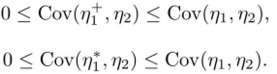
(ii)Let η1≥0,η2be an associated random variable sequence and let ρ>0.If η1≤C0<∞,then

ProofSee Lemmas 4.1 and 4.2 in Birkel[11].
Lemma 4.4Suppose that conditions(A1)(i)-(iii),(A4)and(A5)are satisfied.Then,

where λ is given by(2.4).
ProofTo prove(4.2),we first show that

where

with‖·‖being the L2-norm in Rr.
Obviously,from Lemma 4.2,conditions(A1)(iii)and(A4),

where Astdenotes the(s,t)-element of a matrix A.Then using Corollary 1 in Zhang[16],we have(4.5).

To prove(4.4),it suffices to show that

We first show,for any l∈Rrwith lτl=1,that


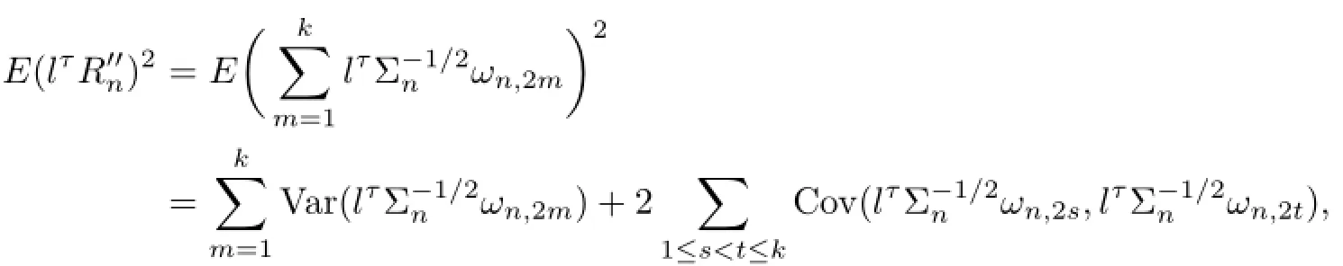
To this end,letlτRncan be split as,where(4.10)follows if we can verify

and by stationarity and(4.8),

where we have used(4.8),Lemma 4.2 and conditions(A1)(iii),(A4).It follows that

which implies(4.12).Similarly,we can prove(4.13).From the proof of(4.15),it can be shown that

Relations(4.16)-(4.17)imply that

Similarly,

Note that Var(lτRn)=1 andUsing(4.18)and(4.19),we have

which implies

Furthermore,by stationarity,(4.8),Lemma 4.2 and conditions(A1)(iii),(A4),we have
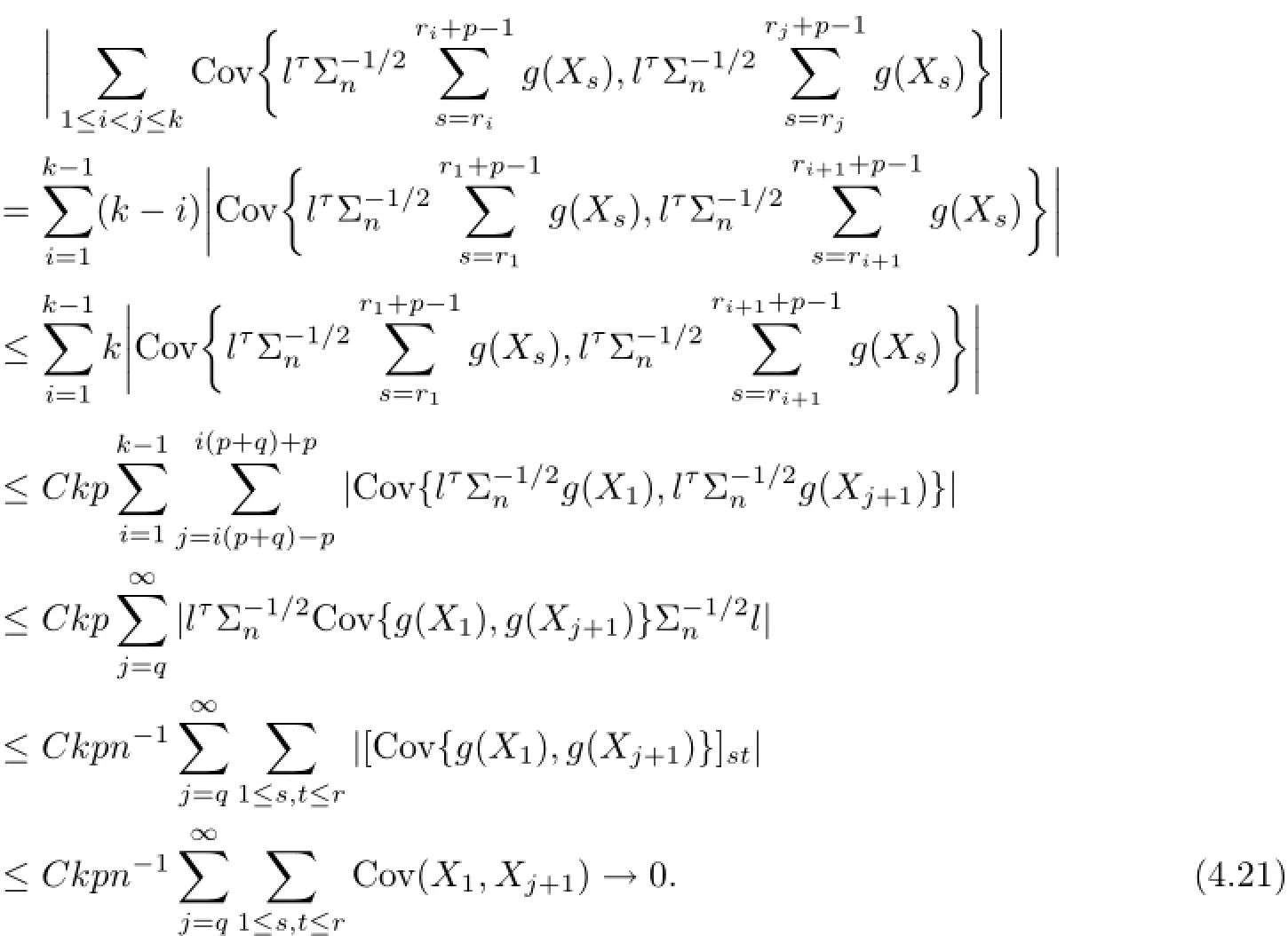
It follows from(4.20)and(4.21)that

which proves(4.14).We thus have(4.10).To prove(4.9),it suffices to show that

Note that where


and

Rewrite lτTn1l as
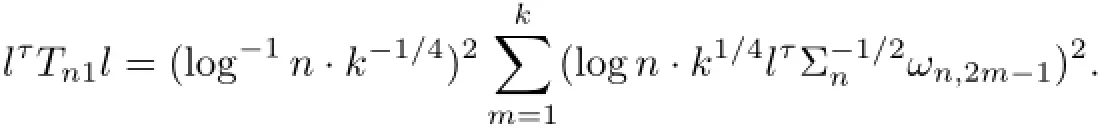

where Firstly,we will show


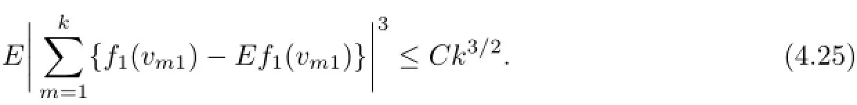
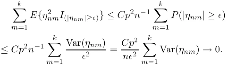
and denote f1(x)=x2I(x≥0),f2(x)=−x2I(x<0).As f1(x)and f2(x)are all monotone functions,{f1(vm1),1≤m≤k},{f2(vm1),1≤m≤k},{f1(vm2),1≤m≤k},{f2(vm2),1≤m≤k},{f1(vm1+vm2),1≤m≤k},and{f2(vm1+vm2),1≤m≤k}are all sequences of PA random variables,and

By contrast,from Lemmas 4.2 and 4.3,similar to the proof of(4.15)in Li et al[17],we have

where we have used condition A5(iii).As E‖g(X)‖6+2δ<∞,δ>0,then by Lemma 4.1,we
have
Similarly,we can show that
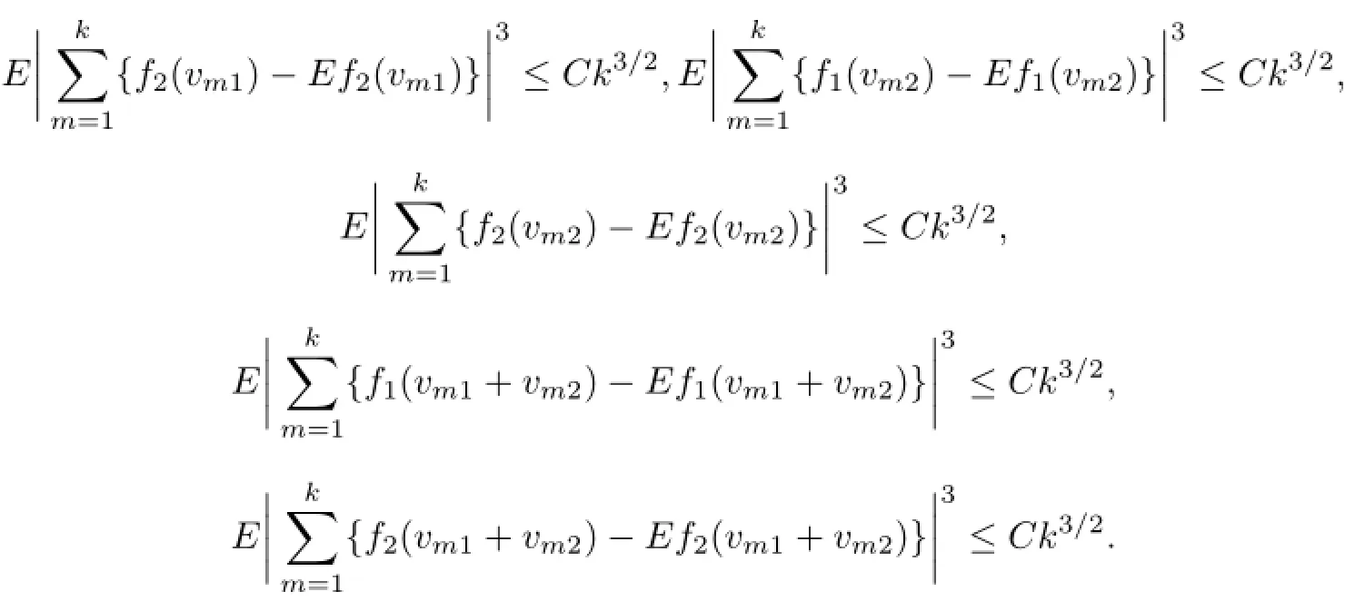
By Cr-inequality,

and(4.23)is thus verified.Similarly,we can prove E|lτTn2l−E(lτTn2l)|3→0 and E|lτTn3l−E(lτTn3l)|3→0.We thus have(4.22).(4.10)and(4.22)implies(4.4).
We now prove(4.2).Let ρ=‖λ‖,λ=ρη.From(2.4),we have
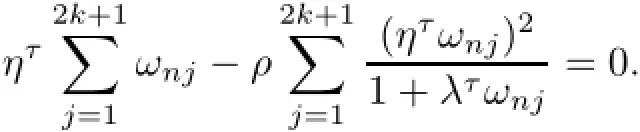
It follows that

where ωnis defined in(4.6).Combining with(4.3)to(4.5),we have ρ/(1+ρωn)=Op(n−1/2). Therefore,


Using(2.4)again,we have

Therefore,combining with(4.4)and(4.5),we may write

where τ is bounded by

The proof of(4.2)is completed.
Lemma 4.5Suppose that conditions(A1)to(A5)are satisfied.Then,for any real-valued sequence yn→θγ,

where

with
ProofProof of(4.27).Similar to the proof of(4.27)and(4.28)in Qin and Lei[8],as yn→θγ,we have

From Lemma 4.2,conditions(A1)(iii),(A2),and(A5),we have

Thus,we have(4.27)from Lemma 1.1 in[16].
Proof of(4.28).Let

By(4.27),to prove(4.28),we only need to show,for any given a∈Rr+1with‖a‖=1,that

with rm=(m−1)(p+q)+1,lm=(m−1)(p+q)+p+1,m=1,···,k.(4.32)follows if we can verify

and

As a preparation,we need to show that

(4.34)-(4.36)can be proved similar to the proofs of(4.12)-(4.14).
We now prove(4.33).Let

where Astdenotes the(s,t)-element of a matrix A.By(4.31),for any a∈Rr+1,is convergent.Thus,uw(q)→0.Similar to the proof of Theorem 2.1 in[9],

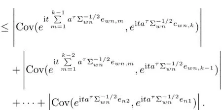
So by Lemma 4.2 and stationarity,we have

Applying the Feller-Lindeberg central limit theorem,we get

(4.33)is thus proved.
Proof of(4.29).Denote

Following the proof of(4.4),we can show that

which leads to(4.29).

The proof of(4.30)is completed.
5 Proof of Theorem 2.1

Next,we will prove

Note that

By conditions(A1)(i),(A1)(iv)and(A2),similar to Lemma 4.3 in Qin and Lei[8],we have

Combining with nh4→0,(4.29),(4.30),(4.2),F(θγ)=γ,and F(yn)−F(θγ)=n−1/2σryf(θγ)+ o(n−1/2),we obtain

Then by(4.28),Cramer-Word theorem,(5.2)and(5.1)lead to Theorem 2.1.
References
[1]Owen A B.Empirical likelihood ratio confidence intervals for a single functional.Biometrika,1988,75:237-249
[2]Owen A B.Empirical likelihood ratio confidence regions.Ann Statist,1990,18:90-120
[3]Chen S X,Hall P.Smoothed empirical likelihood confidence intervals for quantiles.Ann Statist,1993,21:1166-1181
[4]Chen J,Wu C.Estimation of distribution function and quantiles using the model-calibrated pseudo empirical likelihood method.Statist Sinica,2002,12:1223-1239
[5]Kitamura Y.Empirical likelihood methods with weakly dependent processes.Ann Statist,1997,25:2084-2102
[6]Zhang B.M-estimation and quantile estimation in the presence of auxiliary information.J Statist Plann and Inference,1995,44:77-94
[7]Chen J,Qin J.Empirical likelihood estimation for finite populations and the effective usage of auxiliary information.Biometrika,1993,80:107-116
[8]Qin Y,Lei Q.Quantile estimation in the presence of auxiliary information under negatively associated samples.Communications in Statistics-Theory and Method,2011,40:4289-4307
[9]Roussas G G.Asymptotic normality of the kernel estimate of a probability density function under association.Statist Probab Lett,2000,50:1-12
[10]Esary J D,Proschan F,Walkup D W.Association of random variables with applications.Ann Math Statist,1967,38:1466-1474
[11]Birkel T.Moment bounds for associated sequences.Ann Probab,1988,16:1184-1193
[12]Birkel T.On the convergence rate in the central limit theorem for associated processes.Ann Probab,1988,16:1685-1698
[13]Birkel T.A note on the strong law of large numbers for positively dependent random variables.Statist Probab Lett,1989,7:17-20
[14]Bagai I,Prakasa Rao B L S.Kernel-type density and failure rate estimation for associated sequences.Ann Inst Statist Math,1995,47:253-266
[15]Cai Z W,Roussas G G.Smooth estimate of quantiles under associate.Statist.Probab.Lett.1997,36:275-287
[16]Zhang L X.The weak convergence for functions of negatively associated random variables.J Multivariate Anal,2001,78:272-298
[17]Li Y,Qin Y,Lei Q.Confidence intervals for probability density functions under associated samples.J Statist Plann Infer,2012,142:1516-1524
July 11,2014;revised April 10,2015.This work was partially supported by the National Natural Science Foundation of China(11271088,11361011,11201088)and the Natural Science Foundation of Guangxi(2013GXNSFAA019004,2013GXNSFAA019007,2013GXNSFBA019001).
†Corresponding author.
猜你喜欢
天中学刊(2022年3期)2022-11-08
Chinese Physics B(2022年7期)2022-08-01
应用数学(2022年3期)2022-07-07
电子乐园·下旬刊(2021年3期)2021-02-08
太原师范学院学报(社会科学版)(2020年4期)2020-12-22
安全(2020年6期)2020-07-01
作文大王·低年级(2020年4期)2020-04-19
发明与创新·中学生(2019年4期)2019-04-19
北京观察(2016年9期)2017-01-16
校园英语·下旬(2016年3期)2016-04-18
 Acta Mathematica Scientia(English Series)2016年2期
- Acta Mathematica Scientia(English Series)的其它文章
- MEAN-FIELD LIMIT OF BOSE-EINSTEIN CONDENSATES WITH ATTRACTIVE INTERACTIONS IN R2∗
- DIFFERENTIAL OPERATORS OF INFINITE ORDER IN THE SPACE OF RAPIDLY DECREASING SEQUENCES∗
- A BINARY INFINITESIMAL FORM OF TEICHMUüLLER METRIC AND ANGLES IN AN ASYMPTOTIC TEICHMUüLLER SPACE∗
- FAST ALGORITHM FOR CALDER´ON-ZYGMUND OPERATORS:CONVERGENCE SPEED AND ROUGH KERNEL∗
- WEAK TYPE INEQUALITY FOR THE MAXIMAL OPERATOR OF WALSH-KACZMARZ-MARCINKIEWICZ MEANS∗
- ON THE CAUCHY PROBLEM OF A COHERENTLY COUPLED SCHRüODINGER SYSTEM∗