Model analysis of secondary organic aerosol over China with a regional air quality modeling system （RAMS-CMAQ）

LI Ji-Lin， ZHANG Mei-Gen， GAO Yind CHEN Lei

aState Key Laboratory of Atmospheric Boundary Layer Physics and Atmospheric Chemistry （LAPC）， Institute of Atmospheric Physics （IAP），Chinese Academy of Sciences （CAS）， Beijing， China；bCollege of Earth Science， University of Chinese Academy of Sciences， Beijing， China；cCenter for Excellence in Urban Atmospheric Environment， Institute of Urban Environment， Chinese Academy of Sciences， Xiamen， China

Model analysis of secondary organic aerosol over China with a regional air quality modeling system （RAMS-CMAQ）

LI Jia-Lina，b， ZHANG Mei-Gena，c， GAO Yiaand CHEN Leia，b

aState Key Laboratory of Atmospheric Boundary Layer Physics and Atmospheric Chemistry （LAPC）， Institute of Atmospheric Physics （IAP），Chinese Academy of Sciences （CAS）， Beijing， China；bCollege of Earth Science， University of Chinese Academy of Sciences， Beijing， China；cCenter for Excellence in Urban Atmospheric Environment， Institute of Urban Environment， Chinese Academy of Sciences， Xiamen， China

The regional air quality modeling system RAMS-CMAQ was updated to incorporate secondary organic aerosol （SOA） production from isoprene and sesquiterpene and to account for the SOA production rate dependence on NOx and SOA aging. The system was then used to simulate spatiotemporal distributions of SOA concentration and its major constituents over China in winter. Modeled monthly mean SOA concentrations were high in central and eastern China and low in western regions. The highest SOA appeared in regions from Beijing—Tianjin—Hebei （BTH） to the middle reaches of the Yangtze River and areas from Sichuan Basin to the southwest border of China，where SOA contributions were less than 10% of the organic aerosol （OA）. The lowest concentration was in the Qinghai—Tibet Plateau， accounting for 20%—30% of OA. It is notable that contributions from anthropogenic precursors to SOA were signifcant in winter， especially the wide areas of central and eastern China with contributions generally varying from 50% to 80% of the total SOA. Beijing was used as an example location representative of the heavily polluted BTH area for analysis of major components of SOA. Though the modeled concentration of SOA was still underestimated compared to the observations， it still showed that xylene and toluene were the two greatest contributors to anthropogenic SOA， which was in agreement with the observations. SOA produced from monoterpene was the greatest contributor to biogenic SOA due to the high mass yield of monoterpene， followed by isoprene. More than 57% of SOAs were aged， which may increase the extinction efect of SOA.

ARTICLE HISTORY

Revised 17 May 2016

Accepted 24 May 2016

Organic aerosol； haze；Beijing—Tianjin—Hebei； VOCs

为了研究我国二次有机气溶胶（SOA）时空分布及其主要组分，更新了RAMS-CMAQ的SOA模块，主要考虑SOA老化，不同NOx浓度下SOA的形成以及异戊二烯和倍半萜烯生成SOA的机制。结果表明，SOA在我国中东部地区浓度较高而在西部则较低。高SOA覆盖两块区域：京津冀到长江中游及四川盆地到我国西南边界，但对有机气溶胶（OA）的贡献不到10%，低SOA主要出现在青藏高原，占OA的20%—30%。值得注意的是，冬季人为源前体物对SOA的贡献显著，在中东部地区可达50%—80%。在北京，人为源SOA主要前体物是甲苯和二甲苯而单萜烯则是生物源SOA主要前体物。SOA的老化部分超过57%，这可能是SOA消光增强的原因。

1. Introduction

Organic aerosols （OAs） comprise a signifcant fraction（20%—90%） of the total fne particulate mass in the atmosphere （Zhang et al. 2007）. It is well known that OAs signifcantly infuence human health， air quality， and climate change； thus， it has attracted increasing attention in recent years. OAs can be divided into two categories: primary organic aerosol （POA） and secondary organic aerosol （SOA）. POA is emitted directly from anthropogenic and biogenic sources， whereas SOA is formed from the oxidation of volatile or semi-volatile organic compounds（SVOCs） in the atmosphere （Seinfeld and Pankow 2003）. Because of the poor understanding of the various sources，chemical formation and transformation mechanisms， and physicochemical characterization （Hallquist et al. 2009；Zhang et al. 2007）， there are many uncertainties remaining in our knowledge of OAs， among which the formation and evolution of SOAs are the least known.

During the past twenty years， signifcant eforts have been made to investigate SOAs. A number of feld observational studies and laboratory chamber experiments of SOAs have been carried out domestically and abroadto investigate their properties， sources， chemical aging characteristics as well as diurnal and seasonal variations（Cao et al. 2007； Duan et al. 2007； Huang et al. 2014； Riva et al. 2015； Zhang et al. 2008）. Additionally， models have been used to predict spatiotemporal distribution and the properties of SOAs （Fu et al. 2008； Han et al. 2008； Jiang et al. 2012）. However， it has been noted that current atmospheric models underestimate SOA mass. Heald et al. （2005）showed that concentrations of measured organic carbon（OC） over the northwest Pacifc during the ACE-Asia campaign were 10—100 times higher than that simulated by a global chemical transport model with large diferences in SOA estimations. As we can see， the underestimation of SOA in models is still quite common， and the most likely causes are （1） the uncertainty in emission inventories of volatile organic gases； （2） missing precursors， e.g. emissions of semi-volatile organic gases （Robinson et al. 2007）；（3） the exclusion of emissions from regions outside of the studied areas （Jiang et al. 2012）； （4） missing physical/chemical processes that contribute to SOA formation （Fu et al. 2008； Robinson et al. 2007）； and （5） limited model resolution （e.g. Qian， Gustafson， and Fast 2010）.

In order to improve SOA simulation， much work has been conducted. The use of the volatility basis-set （VBS）approach （Donahue et al. 2006）， instead of the traditional two-product method （Odum et al. 1996）， has been a major improvement （Han et al. 2016； Lin et al. 2016）. In their results， the VBS method indeed increased SOA concentrations， but the models do not capture time variation well. So， further understanding and improvement of SOA mechanisms are needed to enhance the performance of SOA simulation.

In this study， RAMS-CMAQ was updated to use the most recent SOA production mechanisms， which include incorporating SOA production from isoprene and sesquiterpene， accounting for SOA production rate dependence on nitrogen oxides and SOA aging. The improved model was applied to investigate the spatiotemporal distributions of SOA concentration as well as its contribution to atmospheric aerosols over China in February 2014.

2. Model description

In this study， CMAQ version 4.7.1 was chosen as the base model and was confgured to use the gas-phase chemical mechanism model SAPRC99 （the 1999 Statewide Air Pollutant Research Center） （Carter 2000）. Compared to previous versions， CMAQ v4.7.1 has been modifed to incorporate two new groups of SOA production pathways:（1） SOA formation from new precursors such as benzene，isoprene， and sesquiterpenes； and （2） SOA formation from new mechanisms， such as NOx-dependent SOA yields from aromatics， acid-catalyzed SOA yields from isoprene， in-cloud SOA formation， and aging of SOA. Furthermore，it allows for the assignment of SOA mass to individual volatile organic compounds （VOCs）.

In this version， SOA is produced from seven VOCs species: long-chain alkanes， high-yield aromatics （toluene），low-yield aromatics （xylene）， benzene， isoprene， monoterpenes and sesquiterpenes. There are 19 secondary organic products during the formation process， of which 12 species are semi-volatile. Semi-volatile VOCs （SVOCs），produced from the oxidation of VOCs， are represented by the two-product model and then absorbed into an organic particulate phase （i.e. semi-volatile SOA） through gas/ particle partitioning behavior （Pankow 1994）. Unlike the semi-volatile SOA， nonvolatile SOA do not partition back to the gas phase. There are four types of nonvolatile SOAs:（1） low-NOx aromatic SOA， （2） acid-enhanced isoprene，（3） oligomers formed through particle-phase reactions，and （4） SOAs from in-cloud oxidation processes. A detailed description was depicted in （Carlton et al. 2010）.

The emission sources used in this model were obtained by several ways. Anthropogenic emissions of VOCs， black carbon （BC）， OC， SO2， NOx， and particle matters were obtained from monthly-based emission inventory of China in 2010 with a spatial resolution of 0.25° × 0.25° and divided into four categories， namely power， industry，residential， and transport （Lu， Zhang， and Streets 2011）. NOxand ammonia from soil were provided by the Global Emissions Inventory Activity （GEIA） 1° × 1° monthly inventory （Benkovitz et al. 1996）. The open biomass burning emissions （from forest wildfres， savanna burning， and agriculture waste burning） were adopted from the Global Fire Emissions Database Version 2 （Randerson et al. 2007）. Besides， emissions of dust and sea salt were estimated online （Gong 2003； Han et al. 2004） in the modeling system.

Our CMAQ model was driven by meteorology felds simulated by RAMS. The model domain was 6654 × 5440 km2for CMAQ （shown in Figure 1） on a rotated polar-stereographic map projection centered at （35°N， 110°E） with a 64-km-grid-cell. The other detailed model confguration information can be found in Han et al. （2014）.

3. Results and discussion

In this study， we chose the month of February 2014 as the modeling period because many places in China experienced heavy haze pollution during this episode， especially the region of Huabei.

3.1. Model evaluation

Figure 1.Geographic locations of CNMC measurement stations in the model domain.

Table 1.Statistical summary of the comparison of the daily average meteorological factors and the hourly PM2.5mass concentrations between observations and simulations at 12 stations in February 2014.

Meteorological factors have important efects on photochemical and aerosol processes. In order to understand the model performance， daily mean meteorological data of 12 stations were used for comparison. The monitoring data from the twelve surface stations （as shown in Figure 1） of the Chinese National Meteorological Center （CNMC） were downloaded from the website （http://www.escience.gov. cn/metdata/page/index.html）.

The observations and model predictions of the daily-average temperature （T）， relative humidity （RH）， wind speed （WS），and direction of maximum wind speed （WD） at the 12 stations in February are presented in the fgures that not shown. RAMS generally predicted the magnitude and day-to-day variation of T， RH， and WS well. As shown in Table 1（a）， average for all 12 stations， the monthly mean observations of T， RH， and WS were 2.74 °C， 67.12%， and 2.21 m s-1， respectively， while mean simulations for these three factors were 2.47 °C， 67.31%，and 2.14 m s-1， respectively. The diferences of the standard deviations of the three factors between measurements and simulations were small. The values of normalized mean bias（NMB） for T， RH， and WS were -9.92%， 0.28%， and -3.10%，respectively， with the correlation coefcients （R） being 0.97，0.84， and 0.62， respectively. However， the simulated directions of maximum wind speed did not coincide well with the observed data. As presented in Table 1（b）， the fraction of samples with an absolute error ≤22.5° between simulation and observation was 29.46%， and the fraction of samples with an absolute error ≤11.25° was 14.28%. The most probable reason is the diferent time resolution （every 10 min for measurements and 1 h for simulations）. Nevertheless， variance of the predicted wind direction was similar to the measurements at most sites with R = 0.53. As a whole， the predicted and measured meteorological data showed good consistency，and the model can reasonably simulate the variations of meteorological phenomena.

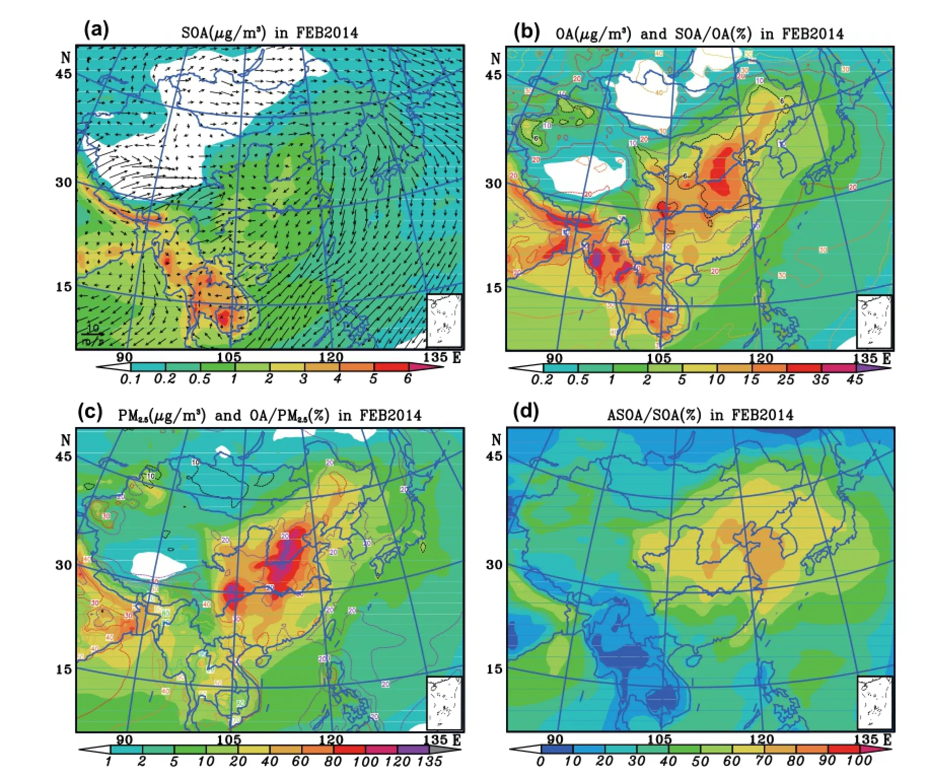
Figure 2.Modeled distributions of monthly mean （a） SOA with wind feld （b） OA （shaded） and SOA/OA （contour line） （c） PM2.5and OA/PM2.5（d） ASOA/SOA in February 2014.

To further evaluate the performance of the model during the period， simulated hourly PM2.5results were compared with the observations provided by the China National Environmental Monitoring Centre （CNEMC）. For all the stations， though simulated values were mostly higher than the observations （with mean bias being approximately 40 μg m-3）， the model had a relatively good ability to capture the variations and trends of fne aerosol mass concentrations. As presented in Table 1（a）， the correlation coefcient was 0.62 between the measurements and simulations， with the standard deviations being 90.72 and 103.86 μg m-3for the observed and predicted concentrations， respectively. Above all， it indicated a generally good ability of the model to predict aerosol concentrations.

3.2. Spatial distribution characteristics of predicted SOA

The OA mass concentrations were simulated in μg m-3，but measured in μgC m-3. For comparison， SOA and OA in Figure 2（a） and （b） were actually SOC and OC.

Figure 2（a） shows the spatial distribution of monthly averaged SOA mass concentration and wind feld. As a whole， in China， the concentration of SOA was high in central and eastern regions and low in the western region. SOA concentration generally varied from 0.5 to 1 μg m-3in central and eastern areas， with maximum （1—2 μg m-3） in portion of regions from the Beijing—Tianjin—Hebei （BTH） area to the middle reaches of the Yangtze River， regions from southeast of Sichuan province to the China—Vietnam border and China—Burma border as well as Hainan Province. The model results were lower than the observed ranges of 3.1—29.9 and 1.4—19.6 μg m-3， respectively （Cao et al. 2007；Dan et al. 2004； Li and Bai 2009； Wang et al. 2015）， due to the uncertainties in the ratio of OC to elemental carbon（EC） when calculating observed SOC， and the underestimation of emission inventories in our model. The simulated SOA concentration in western region of China was less than 0.2 μg m-3， mainly due to low emissions of related precursors. Outside China， in northeast India， central Burma， Thailand and Cambodia etc.， we can also fnd high SOA concentrations （≥3 μg m-3） because of large amountof biomass combustion which may release biogenic VOCs（Rouviere et al. 2006） to produce SOA.

Figure 2（b） presents the spatial distribution of monthly averaged OA mass concentration and the monthly mean fraction of SOA to OA （SOA/OA）. The distribution of OA is similar to SOA: high in the central and eastern regions and low in the western region. The simulated OA concentration was generally in the range of 1—25 μg m-3in central and east China and reached the highest levels （25—35 μg m-3）in the BTH area due to large amount of anthropogenic emissions. The model result in BTH area is comparable to values of （27.2 ± 15.3—38.9 ± 18.4） μg m-3observed by Cao et al. （2007）. OA concentrations in eastern Sichuan Basin were also high （25—35 μg m-3）， within the observed range of （18.3 ± 8.6—76.7 ± 24.6） μg m-3（Cao et al. 2007； Chen et al. 2014）. The reason for the high concentrations is that Sichuan Basin is surrounded by mountains and has some of the lowest wind speeds （Chen and Xie 2012）， which is not conducive to the difusion of pollutants. In addition to the increased carbon emissions from domestic heating and the stable atmospheric conditions， high relative humidity may also contribute to the high OA concentration. In western China， OA concentrations were generally lower than 2 μg m-3， although concentrations in some northwestern areas were 2—10 μg m-3mainly due to relatively high anthropogenic emissions from surrounding areas with dense population. The lowest concentration （≤0.2 μg m-3）appeared in the center of Qinghai—Tibet Plateau resulting from very low source emissions. Outside China， in western Burma， northeastern India and the Thailand—Burma border， we also found high OA concentrations （＞25 μg m-3）because of biomass combustion， including burning of agricultural waste and fuel wood in Southeast Asia.

As illustrated in Figure 2（b）， the SOA fraction ranged from less than 6% to 30% in China， with a relatively higher contribution （generally 10%—30%） in western regions and lower fraction （＜10%） mostly in central and eastern developed areas. The contribution of SOA to OA in south China（6%—20%） and north China （＜10%） were within the range of feld measurements of 6%—60% and 8%—32%， respectively （Cao et al. 2003， 2007； Niu et al. 2006； Zhao， Dong，Yang et al. 2013）. Both the simulated and observed results indicated that the fraction in the north was lower than in the south due to the lower temperatures and reduced sunlight. The lowest fraction （＜6%） mainly appeared in regions where the concentrations of OA were relatively high （e.g. Sichuan Basin and BTH area etc.）. Similarly， in the western regions， the SOA/OA fraction was also the lowest in areas where OA concentration was the highest. This illustrates that emission of POA was the main contributor to high OA. The highest fraction （20%—30%） appeared in Tibet—Qinghai area due to low primary source emissions. Outside China， the SOA fraction was quite large （20%—50%） over wide areas of the western Pacifc Ocean and the northern Indian Ocean due to relatively lower POA emissions and greater oxidation of SOA transported from upwind areas. However， among the areas of high OA concentrations， such as northeast India and central Burma， SOA/OA was less than 20%.

As shown in Figure 2（c）， the distribution of PM2.5mass concentration was also similar to the OA and SOA concentrations. The highest concentration （100—135 μg m-3）occurred in BTH and Sichuan Basin and were within the observed range of （126.5 ± 66.1—179.4 ± 87.8） μg m-3and （158 ± 51—311.8 ± 114.1） μg m-3（Cao et al. 2007； Tao et al. 2014） respectively. The lowest （＜2 μg m-3） occurred in the Tibet—Qinghai Plateau. Outside China， PM2.5in east India was relatively high with the concentration varying from 40 μg m-3to 80 μg m-3due to biomass burning and transportation in the western India with its high fossil fuel consumption and particulate emissions（Reddy and Venkataraman 2002）. As is evident in Figure 2（c）， as a whole， the OA fraction was high in central and eastern China （generally 20%—30%） and low （approximately 10%—20%） in western regions. As a result， the contribution of SOA to PM2.5（SOA/PM2.5） in the areas with low and high concentrations were less than 6% and less than 3%， respectively. Outside China， the OA/PM2.5ratio was the highest in central and south Burma and reached up to 80%—90% due to large amount of biomass burning in these areas.

As presented in Figure 2（d）， because of large amount of anthropogenic VOCs emissions， anthropogenic SOA（ASOA） dominated SOA over wide areas of central and east China （50%—80%） in the winter time， with the fraction reaching more than 60% in the regions from the Huabei plain to the upper reaches of the Yellow River as well as the middle and lower reaches of the Yangtze River. The modeled distribution was similar to that predicted by Jiang et al. （2012）. It was notable that the contribution to SOA from anthropogenic sources was signifcant in the regions of north of the Huabei plain， the Bohai Sea， and the Yellow Sea with contributions up to 80%， resulting from the atmospheric barrier of the Taihang Mountains and transport of clockwise horizontal airfow. The fraction of ASOA to SOA in portions of western remote areas of China can also reach 40%—50% because of the transport of ASOA from neighboring areas. Outside China， the ASOA fraction was also quite high （50%—70%） in eastern India， resulting from the transport from the western India as well as the Himalayas preventing pollutant transmission to the northeast. In the western Pacifc Ocean and the northern Indian Ocean， the fraction of anthropogenic SOA can reach 60%. However， the fraction in south Burma and Cambodia was small （＜10%） because of high biomass burning （Rouviere et al. 2006）.

3.3. Major components of SOA

The BTH area always experiences heavy pollution in winter， so we took Beijing （BJ， 39.8° N， 116.47°E） as an example site to analyze the major components of SOA in this area. SOA was seriously underestimated compared to the observation （0.93 μg m-3vs. 8.66—23.1 μg m-3） with the concentration diference being a multiple of 9.3—24.8 （Dan et al. 2004； Duan et al. 2005； Zhao， Dong， He et al. 2013）. This discrepancy may result from the underestimation of emission inventories in the areas with dense population and high anthropogenic emissions （Liu et al. 2012）. In Beijing， the contribution to SOA from anthropogenic sources was approximately 72.39% with the two most important anthropogenic VOC precursors being xylene and toluene. This is consistent with the observations that the benzene series is one of the main VOCs compounds in the BTH area， with the major constituents including benzene， xylene and toluene （Cao et al. 2012； Jiang et al. 2015；Zhou， Hao， and Wang 2011）. Here， SOA that formed from aromatic compounds （including benzene， xylene， and toluene） accounted for more than 27% of total SOA， which was approximately 6.0 times more than the contribution from long-chain alkanes. Among BSOA components， SOA formed from monoterpenes was the major contributor，followed by that from isoprene， with fractions being 8.74，and 1.27%， respectively. This may result from the higher mass yield from monoterpene （Lane， Donahue， and Pandis 2008）. SOA produced from sesquiterpenes was negligible，with a fraction of approximately 0.04%， probably due to its low emission among biogenic VOCs （Oderbolz et al. 2013）. Aged SOA was produced from oligomerization of SOA in the condensed phase. Its properties， especially the optical property， may change through the aging process. In this study， aged SOA accounted for more than 57% of the total SOA， suggesting the greater extinction of SOA in Beijing，which may give rise to the lower visibility during heavy pollution days.

4. Conclusions

In this study， we used RAMS-CMAQ with the most recent SOA production mechanisms to investigate spatial mass concentration distributions of SOAs as well as their contribution to total atmospheric aerosols over China in February 2014.

In China， the distribution of the mean SOA concentration for the month was similar to OA and PM2.5concentrations， which were high in the central and eastern regions and low in the western region. The highest concentrations were mainly concentrated in the areas around the middle reaches of the Yellow River and the Yangtze River （e.g. BTH area） as well as Sichuan Basin， while the lowest generally occurred in the Qinghai—Tibet Plateau. SOA concentration generally varied from 0.5 μg m-3to 1 μg m-3in the central and eastern areas with maximum concentrations being 1—2 μg m-3， and were not more than 0.2 μg m-3in western China because of low emissions of precursors. Though the high SOA concentration was accompanied by high OA and PM2.5，SOA/OA and SOA/PM2.5in these areas （like BTJ regions and Sichuan Basin） were less than 10% and less than 3%，respectively. SOA/OA， and SOA/PM2.5were 10%—30% and less than 6%， respectively， in the low concentration areas like the Tibet—Qinghai Plateau.

Anthropogenic SOA dominated SOA over wide areas of central and eastern China， with contributions of more than 60%. In portions of the remote western areas of China， the fraction can also reach 40%—50%.

In terms of Beijing， the contribution to SOA from anthropogenic sources was approximately 72.39% with the two greatest contributions coming from xylene and toluene. Among BSOA components， SOA produced from monoterpenes was the major contributor， followed by SOA from isoprene， with fractions of 8.74% and 1.27%， respectively. In this study， aged SOA， produced from oligomerization reactions of SOA， accounted for more than 57%， suggesting the greater extinction efect of SOA.

Disclosure statement

No potential confict of interest was reported by the authors.

Funding

This work was supported by the ‘Strategic Priority Research Program （B）' of the Chinese Academy of Sciences ［XDB05030105］，［XDB05030102］， ［XDB05030103］； the National Basic Research Program of China ［2014CB953802］.

References

Benkovitz， C. M.， M. T. Scholtz， J. Pacyna， L. Tarrason， J. Dignon，E. C. Voldner， P. A. Spiro， J. A. Logan， and T. E. Graedel. 1996.“Global Gridded Inventories of Anthropogenic Emissions of Sulfur and Nitrogen.” Journal of Geophysical Research: Atmospheres 101 （D22）: 29239—29253.

Cao， J. J.， S. C. Lee， K. F. Ho， X. Y. Zhang， S. C. Zou， K. Fung， J. C. Chow，and J. G. Watson. 2003. “Characteristics of Carbonaceous Aerosol in Pearl River Delta Region， China during 2001 Winter Period.” Atmospheric Environment 37 （11）: 1451—1460.

Cao， J. J.， S. C. Lee， J. C. Chow， J. G. Watson， K. F. Ho， R. J. Zhang，Z. D. Jin， et al. 2007. “Spatial and Seasonal Distributions of Carbonaceous Aerosols over China.” Journal of Geophysical Research-Atmospheres 112 （D22）. doi:10.1029/2006jd008205.

Cao， W.， J. Shi， B. Han， X. Wang， Y. Peng， W. Qiu， L. Zhao， and Z. Bai. 2012. “Composition and Distribution of Vocs in the Ambient Air of Typical Cities in Northern of China.” China Environmental Science 32 （2）: 200—206.

Carlton， A. G.， P. V. Bhave， S. L. Napelenok， E. D. Edney， G. Sarwar，R. W. Pinder， G. A. Pouliot， and M. Houyoux. 2010. “Model Representation of Secondary Organic Aerosol in CMAQv4.7.”Environmental Science & Technology 44 （22）: 8553—8560.

Carter， W. P. L. 2000. Implementation of the SAPRC-99 Chemical Mechanism into the Models-3 Framework Report to the US Environmental Protection Agency. Durham， NC: Research Triangle Park.

Chen， Y.， and S. Xie. 2012. “Temporal and Spatial Visibility Trends in the Sichuan Basin， China， 1973 to 2010.” Atmospheric Research 112: 25—34.

Chen， Y.， S. Xie， B. Luo， and C. Zhai. 2014. “Characteristics and Origins of Carbonaceous Aerosol in the Sichuan Basin， China.”Atmospheric Environment 94: 215—223.

Dan， M.， G. S. Zhuang， X. X. Li， H. R. Tao， and Y. H. Zhuang. 2004.“The Characteristics of Carbonaceous Species and Their Sources in PM2.5in Beijing.” Atmospheric Environment 38 （21）: 3443—3452.

Donahue， N. M.， A. L. Robinson， C. O. Stanier， and S. N. Pandis. 2006. “Coupled Partitioning， Dilution， and Chemical Aging of Semivolatile Organics.” Environmental Science & Technology 40 （8）: 2635—2643.

Duan， F. K.， K. B. He， Y. L. Ma， Y. T. Jia， F. M. Yang， Y. Lei， S. Tanaka，and T. Okuta. 2005. “Characteristics of Carbonaceous Aerosols in Beijing， China.” Chemosphere 60 （3）: 355—364.

Duan， J.， J. Tan， D. Cheng， X. Bi， W. Deng， G. Sheng， J. Fu， and M. H. Wong. 2007. “Sources and Characteristics of Carbonaceous Aerosol in Two Largest Cities in Pearl River Delta Region， China.”Atmospheric Environment 41 （14）: 2895—2903.

Fu， T.-M.， D. J. Jacob， F. Wittrock， J. P. Burrows， M. Vrekoussis，and D. K. Henze. 2008. “Global Budgets of Atmospheric Glyoxal and Methylglyoxal， and Implications for Formation of Secondary Organic Aerosols.” Journal of Geophysical Research-Atmospheres 113 （D15）. doi:10.1029/2007jd009505.

Gong， S. L. 2003. “A Parameterization of Sea-Salt Aerosol Source Function for Sub- and Super-micron Particles.” Global Biogeochemical Cycles 17 （4）. doi:10.1029/2003gb002079.

Hallquist， M.， J. C. Wenger， U. Baltensperger， Y. Rudich，D. Simpson， M. Claeys， J. Dommen， et al. 2009. “The Formation，Properties and Impact of Secondary Organic Aerosol: Current and Emerging Issues.” Atmospheric Chemistry and Physics 9（14）: 5155—5236.

Han， Z. W.， H. Ueda， K. Matsuda， R. J. Zhang， K. Arao， Y. Kanai， and H. Hasome. 2004. “Model Study on Particle Size Segregation and Deposition during Asian Dust Events in March 2002.”Journal of Geophysical Research-Atmospheres 109 （D19）. doi:10.1029/2004jd004920.

Han， Z.， R. Zhang， and Q. G. Wang， W. Wang， J. Cao， and J. Xu. 2008. “Regional Modeling of Organic Aerosols over China in Summertime.” Journal of Geophysical Research-Atmospheres 113 （D11）. doi:10.1029/2007jd009436.

Han， X.， M. Zhang， J. Gao， S. Wang， and F. Chai. 2014. “Modeling Analysis of the Seasonal Characteristics of Haze Formation in Beijing.” Atmospheric Chemistry and Physics 14 （18）: 10231—10248.

Han， Z.， Z. Xie， G. Wang， R. Zhang， and J. Tao. 2016. “Modeling Organic Aerosols over East China Using a Volatility Basis-set Approach with Aging Mechanism in a Regional Air Quality Model.” Atmospheric Environment 124: 186—198.

Heald， C. L.， D. J. Jacob， R. J. Park， L. M. Russell， B. J. Huebert，J. H. Seinfeld， H. Liao， and R. J. Weber. 2005. “A Large Organic Aerosol Source in the Free Troposphere Missing from Current Models.” Geophysical Research Letters 32 （18）. doi:10.1029/ 2005gl023831.

Huang， R.-J.， Y. Zhang， C. Bozzetti， K.-F. Ho， J.-J. Cao， Y. Han，K. R. Daellenbach， et al. 2014. “High Secondary Aerosol Contribution to Particulate Pollution during Haze Events in China.” Nature 514 （7521）: 218—222.

Jiang， F.， Q. Liu， X. Huang， T. Wang， B. Zhuang， and M. Xie. 2012.“Regional Modeling of Secondary Organic Aerosol over China Using WRF/Chem.” Journal of Aerosol Science 43 （1）: 57—73.

Jiang， J.， W. Jin， L. Yang， Y. Feng， Q. Chang， Y. Li， and J. Zhou. 2015.“The Pollution Characteristic of Vocs of Ambient Air in Winter in Shijiazhang.” Environmental Monitoring in China 31 （1）: 79—84.

Lane， T. E.， N. M. Donahue， and S. N. Pandis. 2008. “Simulating Secondary Organic Aerosol Formation Using the Volatility Basis-set Approach in a Chemical Transport Model.”Atmospheric Environment 42 （32）: 7439—7451.

Li， W.， and Z. Bai. 2009. “Characteristics of Organic and Elemental Carbon in Atmospheric Fine Particles in Tianjin， China.”Particuology 7 （6）: 432—437.

Lin， J.， J. An， Y. Qu， Y. Chen， Y. Li， Y. Tang， F. Wang， and W. Xiang. 2016. “Local and Distant Source Contributions to Secondary Organic Aerosol in the Beijing Urban Area in Summer.”Atmospheric Environment 124: 176—185.

Liu， Z.， Y. Wang， M. Vrekoussis， A. Richter， F. Wittrock， J. P. Burrows，M. Shao， et al. 2012. “Exploring the Missing Source of Glyoxal（Chocho） over China.” Geophysical Research Letters 39. doi:10.1029/2012gl051645.

Lu， Z.， Q. Zhang， and D. G. Streets. 2011. “Sulfur Dioxide and Primary Carbonaceous Aerosol Emissions in China and India，1996—2010.” Atmospheric Chemistry and Physics 11 （18）: 9839—9864.

Niu， Y.， L. He， M. Hu， J. Zhang， and Y. Zhao. 2006. “Pollution Characteristics of Atmospheric Fine Particles and Their Secondary Components in the Atmosphere of Shenzhen in Summer and in Winter.” Science in China Series B-Chemistry 49（5）: 466—474.

Oderbolz， D. C.， S. Aksoyoglu， J. Keller， I. Barmpadimos，R. Steinbrecher， C. A. Skjoth， C. Plass-Duelmer， and A. S. H. Prevot. 2013. “A Comprehensive Emission Inventory of Biogenic Volatile Organic Compounds in Europe: Improved Seasonality and Land-cover.” Atmospheric Chemistry and Physics 13 （4）: 1689—1712.

Odum， J. R.， T. Hofmann， F. Bowman， D. Collins， R. C. Flagan， and J. H. Seinfeld. 1996. “Gas/Particle Partitioning and Secondary Organic Aerosol Yields.” Environmental Science & Technology 30 （8）: 2580—2585.

Pankow， J. F. 1994. “An Absorption-model of Gas-particle Partitioning of Organic-compounds in the Atmosphere.”Atmospheric Environment 28 （2）: 185—188.

Qian， Y.， W. I. Gustafson Jr.， and J. D. Fast. 2010. “An Investigation of the Sub-grid Variability of Trace Gases and Aerosols for Global Climate Modeling.” Atmospheric Chemistry and Physics 10 （14）: 6917—6946.

Randerson， J. T.， G. R. van der Werf， L. Giglio， G. J. Collatz，and P. S. Kasibhatla. 2007. Global Fire Emissions Database，Version 2 （GFEDv2.1）. Oak Ridge， TN: Oak Ridge National Laboratory Distributed Active Archive Center. doi:10.3334/ ORNLDAAC/849.

Reddy， M. S.， and C. Venkataraman. 2002. “Inventory of Aerosol and Sulphur Dioxide Emissions from India: I — Fossil Fuel Combustion.” Atmospheric Environment 36 （4）: 677—697.

Riva， M.， E. S. Robinson， E. Perraudin， N. M. Donahue， and E. Villenave. 2015. “Photochemical Aging of Secondary Organic Aerosols Generated from the Photooxidation of Polycyclic Aromatic Hydrocarbons in the Gas-phase.”Environmental Science & Technology 49 （9）: 5407—5416.

Robinson， A. L.， N. M. Donahue， M. K. Shrivastava， E. A. Weitkamp，A. M. Sage， A. P. Grieshop， T. E. Lane， J. R. Pierce， and S. N. Pandis. 2007. “Rethinking Organic Aerosols: Semivolatile Emissions and Photochemical Aging.” Science 315 （5816）: 1259—1262.

Rouviere， A.， G. Brulfert， P. Baussand， and J. P. Chollet. 2006.“Monoterpene Source Emissions from Chamonix in the Alpine Valleys.” Atmospheric Environment 40 （19）: 3613—3620. Seinfeld， J. H.， and J. F. Pankow. 2003. “Organic Atmospheric Particulate Material.” Annual Review of Physical Chemistry 54: 121—140.

Tao， J.， J. Gao， L. Zhang， R. Zhang， H. Che， Z. Zhang， Z. Lin， J. Jing，J. Cao， and S. C. Hsu. 2014. “PM2.5Pollution in a Megacity of Southwest China: Source Apportionment and Implication.”Atmospheric Chemistry and Physics 14 （16）: 8679—8699.

Wang， J.， S. S. H. Ho， J. Cao， R. Huang， J. Zhou， Y. Zhao， H. Xu， et al. 2015. “Characteristics and Major Sources of Carbonaceous Aerosols in PM2.5from Sanya， China.” Science of the Total Environment 530: 110—119.

Zhang， Q.， J. L. Jimenez， M. R. Canagaratna， J. D. Allan，H. Coe， I. Ulbrich， M. R. Alfarra， et al. 2007. “Ubiquity and Dominance of Oxygenated Species in Organic Aerosols in Anthropogenically-Infuenced Northern Hemisphere Midlatitudes.” Geophysical Research Letters 34 （13）. doi:10.10 29/2007gl029979.

Zhang， X. Y.， Y. Q. Wang， X. C. Zhang， W. Guo， and S. L. Gong. 2008.“Carbonaceous Aerosol Composition over Various Regions of China during 2006.” Journal of Geophysical Research-Atmospheres 113 （D14）. doi:10.1029/2007jd009525.

Zhao， P.， F. Dong， Y. Yang， D. He， X. Zhao， W. Zhang， Q. Yao， and H. Liu. 2013. “Characteristics of Carbonaceous Aerosol in the Region of Beijing， Tianjin， and Hebei， China.” Atmospheric Environment 71: 389—398.

Zhao， P. S.， F. Dong， D. He， X. J. Zhao， X. L. Zhang， W. Z. Zhang，Q. Yao， and H. Y. Liu. 2013. “Characteristics of Concentrations and Chemical Compositions for PM2.5in the Region of Beijing，Tianjin， and Hebei， China.” Atmospheric Chemistry and Physics 13 （9）: 4631—4644.

Zhou， Y.， Z. Hao， and H. Wang. 2011. “Pollution and Source of Atmospheric Volatile Organic Compounds in Urban-rural Juncture Belt Area in Beijing.” Chinese Journal of Environmental Science 32 （12）: 3560—3565.

有机气溶胶； 灰霾； 京津冀；挥发性有机化合物

31 March 2016

CONTACT ZHANG Mei-Gen mgzhang@mail.iap.ac.cn

© 2016 The Author（s）. Published by Informa UK Limited， trading as Taylor & Francis Group.

This is an Open Access article distributed under the terms of the Creative Commons Attribution License （http://creativecommons.org/licenses/by/4.0/）， which permits unrestricted use， distribution， and reproduction in any medium， provided the original work is properly cited.