
Global Stability of A Stochastic Predator-prey Model with Stage-structure
2017-03-14 02:46
(Basic Department of Military and Politics,Army Engineering University of PLA,Shijiazhuang campus,Shijiazhuang 050003,P.R.China)
§1.Introduction
Since the pioneer work of Lotka and Volterra on predator-prey system,variants of the Lotka-Volterra equations have been frequently used to describe population dynamics with predatorprey relations.In order to reflect the nature of the competitive interactions and predator-prey relationships between them,many tools have been used.Such as stage structure,response function,time delay,prey refuge etc.[1-5].Moveover,the species are exposed to the impact of a large number of random unpredictable factors,so it is necessary and important to consider the corresponding stochastic population model[6-8].
The classical Bazykin’s model[9]can be written as
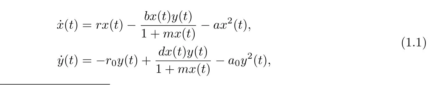
wherer0is the natural death rate of the predator,a0is the intra-specific competition ratio of the predator.
Observing the importance of stage structure,we are influenced to modify the classical Bazykin’s model by taking into this factor.And thus the system(1.1)takes the following form:
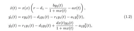
wherex(t),y1(t),y2(t)denote the densities of the prey,the immature predator and the mature predator,respectively.r,eare the intrinsic growth rates of prey and immature predator,respectively.d,d1,d2are the natural death rates of the prey,immature predator and the mature predator,respectively.a,a1,a2are the intra-specific competition ratios of the prey,immature predator and the mature predator,respectively.bis the capturing rate,d/bis the conversion rate of the mature predator,mis the half capturing saturation constant,r1denotes the rate of immature predator becoming mature predator.
Now let us take a further consideration by taking the environmental noise into account.
Firstly,ifa<m(r−d1),>0 hold,then system(1.2)has positive equilibrium(x∗,).Secondly,recall thatd,d1,d2represent the death rates,we replace these parameters by some random parameters,which is a way to model the effect of the environmental fluctuations[10-11].We can replace the death rates by an average value plus random fluctuation terms:

Then corresponding deterministic model system(1.2),the stochastic system takes the following form
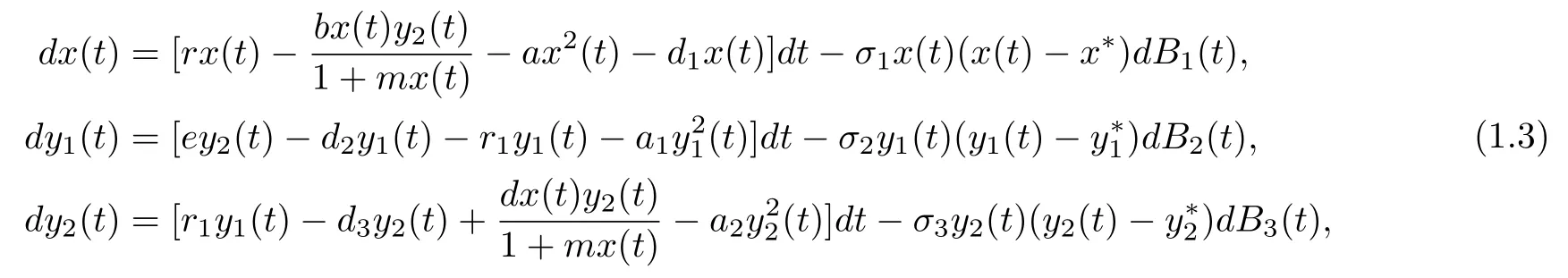
where(i=1,2,3)represents the intensity of the noise and(t)is a standard white noise,namelyBi(t)is a standard Brownian motion defined on a complete probability space(Ω,F,P)with a filtration{Ft}t∈R+satisfying the usual conditions(i.e.it is right continuous and increasing whileF0contains allP-null sets).
The initial conditions for system(1.3)takes the formx(0),y1(0),y2(0)>0.
The organization of this paper is as follows.In Sec.2,by Itˆo′s formula,we establish the sufficient conditions for global asymptotic stability of system(1.3).In Sec.3,we numerically simulate the solution of the system(1.3)to illustrate the results above.
§2.Global Stability
In this section,we firstly give some conditions which system(1.3)has a global positive solution.Then establish the sufficient conditions for global asymptotic stability of system(1.3).
Similar to Liu and Wang[12],we have the following Lemma.
Lemma 2.1For any giver initial value(x(0),y1(0),y2(0))system(1.3)has a unique positive solution(x1(t),y1(t),y2(t))ont≥0 almost surely(a.s.),where={x∈R3|xi>0,i=1,2,3}.
Next,we give the main result of this paper.
Theorem 2.1If(H1):A1>0,A2>0,A3>0 hold,where
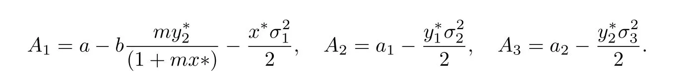
Then the equilibrium position(x∗,)of system(1.3)is globally asymptotical stable with probability 1,i.e.for any initial data(x(0),y1(0),y2(0)),then the solution of system(1.3)has the property that limt→+∞(x(t),y1(t),y2(t))=(x∗,,)a.s.i=1,2,3.
ProofFrom the stability theory of stochastic differential equations,we only need to find a Lyapunov functionV(z)satisfyingLV(z)≤0 with equality if and only ifz=z∗(see e.g[11]),wherez=z(t)is the solution of the n-dimensional stochastic differential equation

z∗is the equilibrium position of(2.1),andLV(z)=Vz(z)f(t,z)+0.5trace[gT(t,z)Vzz(z)g(t,z)].
System(1.3)can be rewritten as
whereci>0,i=1,2,3 are determined.
Clearly,if(H1)holds,then Eq.(2.6)implies thatLV(x)<0 along all trajectories inexcept(x∗,).So the desired assertion follows immediately.
Now,let us return back to system(1.2).We can get the following result.
Corollary 2.1Ifa>(1.2)is globally asymptotically stable.
Remark 1By comparing Theorem 2.1 with Corollary 2.1,we can see that if the positive equilibrium of the deterministic model is globally stable,then the stochastic system will keep this property well when the noise is enough small.
§3.Numerical Simulation
In order to con firm the results above,we numerically simulate the solution of system(1.3)theoretical analysis.
We will use the Milstein method mentioned in Higham[13]to substantiate the analytical findings.For system(1.3),consider the discretization equation:

whereξk,,are the Gaussian random variables which followN(0,1).
To show the global asymptotical stability of the stochastic predator-prey system(1.3)atE∗,we choose a set of parametersr=1.1,d1=0.5,b=0.5,m=0.5,a=0.1,e=2.5,d2=0.2,r1=0.3,a1=0.3,d3=0.3,d=0.9,a2=0.5,and with initial value(0.5,0.5,0.5).It is easy to obtain the positive equilibriumE∗=(1.3576,2.8653,1.5588).
We can see the globally asymptotical stability of the deterministic system(1.2)from Fig.1.In order to show the the globally asymptotical stability the stochastic system(1.3),we can chooseσ1=0.4,σ2=0.2,σ3=0.2,by virtue of Theorem 2.1,the equilibrium positionE∗of system(1.3)is globally asymptotically stable.See Fig.2.When we chooseσ1=0.8,σ2=0.7,σ3=0.7,which violate the condition(2.1).From the Fig.3.we can see that all the species die out.By comparing the Fig.1 and Fig.3,we can conclude that if the positive equilibrium of the deterministic system is globally stable,then the stochastic model will preserve this property when the noise is suitable.
§4.Discussion
Considering the theoretical and practical significance,predator-prey system has been studied a lot.However,the environmental noises always have effect on the predator-prey system.It is necessary to consider the corresponding stochastic system.In this paper,we considered a stochastic predator-prey system with ratio-dependent response function and stage structure for predator.We aimed to reveal how death rates ofx(t),y1(t),y2(t)under random perturbation took effect on the global stability of system(1.2).Some sufficient conditions for global asymptotical stability were established.In biological point of view,it means that the community consisting of two species is a stable biotic community in which all species will coexist.

Figure 1:The positive solution E∗ found by numerical integration of system(1.3)with σ1=0,σ2=0,σ3=0.(a),(b)and(c)are x,y1,y2versus t,respectively.(d)is the projected x−y1−y2 phase plane.
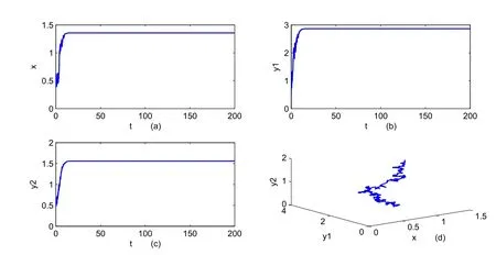
Figure 2:The positive solution E∗ found by numerical integration of system(1.3)with σ1=0.4,σ2=0.2,σ3=0.2.(a),(b)and(c)are x,y1,y2versus t,respectively.(d)is the projected x−y1−y2phase plane.
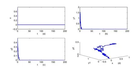
Figure 3:The positive solution E∗ found by numerical integration of system(1.3)with σ1=0.8,σ2=0.7,σ3=0.7.(a),(b)and(c)are x,y1,y2versus t,respectively.(d)is the projected x−y1−y2phase plane.
[1]Kuang Yang.Delay Differential Equations with Applicaiton in Population Dynamics[M].New York:Academic Press,1993,2-15.
[2]GOPALSWAMY K.Stability and Oscillations in Delay Differential Equations of Population Dynamics[M].Dordrecht:Kluwer Academic Press,1992,21-46.
[3]SATIO Y,TAKEUCHI Y.A time-delay model for prey-predator growth with stage structure[J].J of Can Appl Math Quar,2003,11(1):293-302.
[4]JANA S,CHAKRABORTY M,CHAKRABORTY K,et al.,.Global stability and bifurcation of time delayed prey-predator system incorporating prey refuge[J].J of Math Comput Simul,2012,85(3):57-77.
[5]HUANG Ji-cai,XIAO Dong-mei.Analyses of bifurcation and stability in a predator-prey system with Holling type-IV functional response[J].J of Acta Mathematicae Applicaiton Sinica,English Series,2004,20(1):167-178.
[6]JI Chun-yan,JIANG Da-qing,SHI Ning-zhongs.A note on a predator-prey model with modified Leslie-Gower and Holling-type II schemes with stochastic perturbation[J].J of Math Anal Appl,2011,377(1):435-440.
[7]Mandal P S,BANERJEE M.Stochastic persistence and stationary distribution in a Holling-Tanner type prey-predator model[J].J of Physica A,2012,391(4):1216-1233.
[8]JI Chun-yan,JIANG Da-qing.Dynamics of a stochastic density dependent predator-prey system with Bdddigton-DeAngelis functional response[J].J of Math Anal Appl,2011,381(1):441-453.
[9]BAZYKIN A D.Non-linear dynamic of interacting population.In:Chua,L.O.(ed.)Series on Non Linear Science,Series A,vol.11.World Scietific,Singapore,1985.Original Russian version:Bazykin,A.D.,Nauka,Moscow,1998.
[10]GARD T C.Stability for multispecies population models in random environments[J].J of Nonlinear Anal,1986,10(12):1411-1419.
[11]MAO Xue-rong,YUAN Cheng-gui,ZOU Jie-zhong.Stochastic differential delay equations of population dynamics[J].J of Math Anal Appl,2005,304(1):108-119.
[12]LIU-Meng,WANG-Ke.Global stability of a nonlinear stochastic predator-prey system with Bedding-DeAngelis functional response[J].J of Commun Nonlinear Sci Numer Simular,2011,16(3):1114-1121.
[13]HIGHAM D J.An algorithmic intorduction to numerical simulation of stochastic differential equations[J].J of Siam Rev 2001,43(3):525-546.
 Chinese Quarterly Journal of Mathematics2017年4期
- Chinese Quarterly Journal of Mathematics的其它文章
- Local Existence of Solution to the Incompressible Oldroyd Model Equations
- A Finite Volume Unstructured Mesh Method for Fractional-in-space Allen-Cahn Equation
- General Integral Formulas of(0,q)(q>0)Differential Forms on the Analytic Varieties
- The 1-Good-neighbor Connectivity and Diagnosability of Locally Twisted Cubes
- Adjacent Vertex Distinguishing I-total Coloring of Outerplanar Graphs
- Recover Implied Volatility in Short-term Interest Rate Model